Testing the last observation for instability

library(proxymix)

has_ggplot2 <- requireNamespace("ggplot2", quietly = TRUE)

The problem

Suppose you follow a series over time, such as monthly sales, and you have a model fitted to every value so far. One new value has just arrived. You want to know whether it is consistent with the model, or whether something has changed.

Most tests for a change in a series need data on both sides of the change. The breakpoint test of Chow (1960) and the sup-Wald test of Andrews (1993), which tries every possible change point, estimate the model before and after a change and compare the two. With one new value, or a handful, the model after the change cannot be estimated. Chow (1960) also proposed a predictive test that works in this case, but it assumes that the errors follow a normal distribution (Andrews, 2003).

Andrews (2003) proposed end-of-sample tests for exactly this case. proxymix implements a version of them for state-space models. These models describe a series through an unobserved state, such as a level, that changes over time.

Package capabilities

gmm_filter() runs the Kalman filter, which tracks the unobserved state of a series one time step at a time. Before each new value arrives, the filter forecasts it. The difference between the value and its forecast is called the innovation.
gmm_eos_test() tests whether the last m values of a series are consistent with the model. It takes the model in the same form as gmm_filter(). It returns a p-value, a decision at the 5% level, and the numbers used to compute them.

The test statistic is built from the innovations. Each innovation is divided by its standard deviation, which the filter also reports. If the model is correct and nothing has changed, the result, $z_t$ , follows a standard normal distribution. The statistic adds up the squares of the last m of them: $\mathrm{EoS}_m = \sum_{t = n-m+1}^{n} z_t^2.$ A change in the last m values makes their forecasts worse and the statistic larger.

gmm_eos_test() offers two ways, or calibrations, of turning the statistic into a p-value.

method = "chisq", the default, compares the statistic with a chi-square distribution, the distribution of a sum of squared standard normal values. Its degrees of freedom, the number of squared values in the sum, are m times the number of variables observed at each time step. The p-value is exact when the innovations are normal and the model’s parameters are known.
method = "andrews" compares the statistic with the same statistic computed on every earlier block of m consecutive values of the series. The p-value is the share of blocks at least as large as the final block, counting the final block itself. Taking p-values from the data in this way is called subsampling. It follows the P-test of Andrews (2003), with two differences: the p-value counts the tested block, and the earlier blocks are computed from the supplied model rather than from a model re-estimated without each block.

The subsampling calibration does not assume normal innovations. It does make other assumptions. Its p-value is valid only as the series grows long with m fixed, and only if the innovations before the tested block are stationary, meaning that their distribution does not change over time. Its size in a short series can differ from nominal in either direction: the discreteness of the p-value makes it conservative at m = 1 with the model’s parameters known, but it can reject too often when the blocks are no longer exchangeable, such as with estimated parameters or the overlapping blocks of m > 1.

Addressing the problem

set.seed(20260621)

A model and a stable series

The model is a local-level model. An unobserved level moves as a random walk, taking a small normal step at each time point. Each observation is the level plus normal noise. In gmm_filter() form, the prior gives the starting level, dynamics gives the steps of the level, and measurement gives the noise of the observations. gmm() builds a mixture of normal distributions, and with weights = 1 it is a single normal distribution. A prior variance of 10 means the starting level is known only roughly.

prior <- gmm(weights = 1, means = list(0), covariances = list(matrix(10)))
dynamics <- list(A = matrix(1), Q = matrix(0.04))  # the level's random walk
measurement <- list(C = matrix(1), R = matrix(1))  # the observation noise

n <- 120L
level <- cumsum(c(0, rnorm(n - 1L, 0, sqrt(0.04))))
y_stable <- level + rnorm(n, 0, 1)

The same series with a broken final value

A copy of the series has its final value moved up by five standard deviations of the observation noise. Both series are tested at m = 1 with the subsampling calibration.

y_break <- y_stable
y_break[n] <- y_break[n] + 5

test_stable <- gmm_eos_test(
  prior, dynamics, measurement, y_stable, m = 1L, method = "andrews"
)
test_break <- gmm_eos_test(
  prior, dynamics, measurement, y_break, m = 1L, method = "andrews"
)

The end-of-sample test on the same series before and after its final value is moved up by five standard deviations of the observation noise.
Result	Stable series	Broken final value
statistic	0.085	23.194
p-value	0.7417	0.0083
reject at 0.05	FALSE	TRUE
calibration	andrews	andrews
window m	1	1

What the filter expected

The figure shows the forecasts behind the statistic. Before each value arrives, the filter forecasts it from the values before it. The shaded band spans two forecast standard deviations either side of each forecast. The statistic divides each innovation by this forecast standard deviation.

filtered <- gmm_filter(
  prior, dynamics, measurement, y_stable, ridge_eps = 0
)
# ridge_eps adds a tiny amount to each covariance for numerical stability;
# 0 keeps the filter's recursion exact
path <- filtered$summary
# forecast of y_t and its standard deviation, from the filter at t - 1
pred_mean <- c(prior@means[[1L]], path$mean_1[-n])
pred_sd <- sqrt(c(prior@covariances[[1L]][1L, 1L], path$sd_1[-n]^2) +
                  dynamics$Q[1L, 1L] + measurement$R[1L, 1L])
outside <- sum(abs(y_stable - pred_mean)[-1L] > 2 * pred_sd[-1L])

series_df <- data.frame(
  t = seq_len(n),
  observed = y_stable,
  truth = level,
  filtered = path$mean_1,
  lo = pred_mean - 2 * pred_sd,
  hi = pred_mean + 2 * pred_sd
)
break_df <- data.frame(t = n, y = y_break[n])
ggplot2::ggplot(series_df, ggplot2::aes(t)) +
  ggplot2::geom_ribbon(
    data = series_df[-1L, ], ggplot2::aes(ymin = lo, ymax = hi),
    fill = "#0072B2", alpha = 0.18
  ) +
  ggplot2::geom_point(
    ggplot2::aes(y = observed, colour = "observed (stable)"),
    size = 1.1, alpha = 0.7
  ) +
  ggplot2::geom_line(
    ggplot2::aes(y = truth, colour = "true level"), linewidth = 0.8
  ) +
  ggplot2::geom_line(
    ggplot2::aes(y = filtered, colour = "estimated level"), linewidth = 0.8
  ) +
  ggplot2::geom_point(
    data = break_df, ggplot2::aes(t, y, colour = "broken final value"),
    size = 2.6
  ) +
  ggplot2::scale_colour_manual(
    name = NULL,
    values = c(
      "observed (stable)" = "grey60",
      "true level" = "#009E73",
      "estimated level" = "#0072B2",
      "broken final value" = "#D55E00"
    )
  ) +
  ggplot2::labs(
    x = "time step", y = "observation",
    title = "A break in the last observation"
  ) +
  ggplot2::theme_minimal(base_size = 11) +
  ggplot2::theme(legend.position = "top")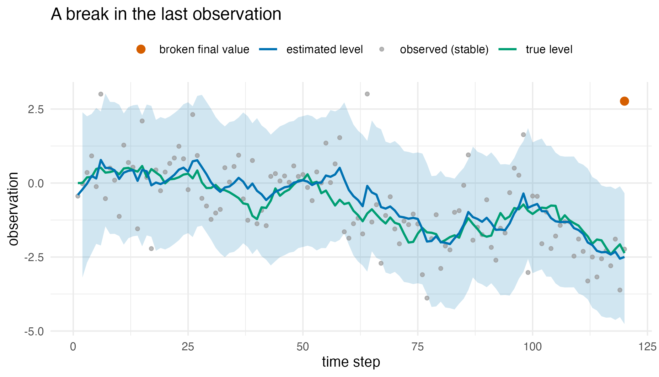

A time series of noisy observations in grey with the true and estimated level overlaid, a shaded forecast band around them, and a single isolated point at the right-hand end lying well above the band.

The simulated series, the unobserved level that generated it, the level estimated by the filter, and a band of two forecast standard deviations either side of each forecast. The band starts at the second time step. The broken final value lies far outside the band.

How the subsampling p-value is reached

The subsampling calibration ranks the final block among the earlier blocks of the same series. The next figure shows that ranking for both series.

blocks_df <- rbind(
  data.frame(
    block = test_stable$in_sample_blocks, series = "stable series"
  ),
  data.frame(
    block = test_break$in_sample_blocks, series = "broken final value"
  )
)
blocks_df$series <- factor(
  blocks_df$series, levels = c("stable series", "broken final value")
)
rule_df <- data.frame(
  series = factor(
    c("stable series", "broken final value"),
    levels = c("stable series", "broken final value")
  ),
  statistic = c(test_stable$statistic, test_break$statistic)
)
ggplot2::ggplot(blocks_df, ggplot2::aes(block)) +
  ggplot2::stat_ecdf(geom = "step", linewidth = 0.8, colour = "#0072B2") +
  ggplot2::geom_vline(
    data = rule_df, ggplot2::aes(xintercept = statistic),
    colour = "#D55E00", linetype = "dashed", linewidth = 0.8
  ) +
  ggplot2::facet_wrap(~ series) +
  ggplot2::scale_x_log10(labels = function(v) {
    format(v, scientific = FALSE, drop0trailing = TRUE, trim = TRUE)
  }) +
  ggplot2::labs(
    x = "block statistic (log scale)",
    y = "cumulative share of earlier blocks",
    title = "The final block against the earlier blocks of the same series"
  ) +
  ggplot2::theme_minimal(base_size = 11)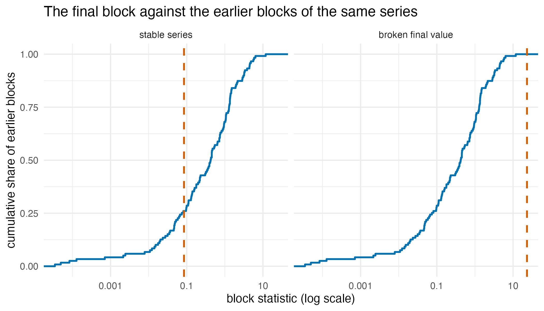

Two panels, each showing a rising step function of the cumulative share of earlier block statistics against a logarithmic axis, with a dashed vertical line. In the left panel the line falls inside the curve. In the right panel it lies far beyond the curve's right-hand end.

The cumulative distribution of the earlier block statistics in each series, with the final block’s statistic as a dashed line. The p-value is $(1 + k) / (n - 2m + 2)$ , where $k$ is the number of earlier blocks at or beyond the dashed line. The stable series’ final block lies inside the range of earlier blocks. The broken series’ final block lies beyond every earlier block.

How often each calibration rejects when the model is known

The size of a test is how often it rejects when nothing has changed. A test at the 5% level should have a size of 0.05. The chunk below simulates stable series of 30 values from the same model, tests each one, and records the share of p-values below 0.05. The model’s parameters are known here, as in the example above.

simulate_null <- function(n_obs) {
  lv <- cumsum(c(0, rnorm(n_obs - 1L, 0, sqrt(0.04))))
  lv + rnorm(n_obs, 0, 1)
}
empirical_size <- function(n_obs, method, n_rep) {
  p <- vapply(seq_len(n_rep), function(i1) {
    gmm_eos_test(
      prior, dynamics, measurement, simulate_null(n_obs),
      m = 1L, method = method
    )$p_value
  }, numeric(1L))
  size <- mean(p < 0.05)
  c(size = size, se = sqrt(size * (1 - size) / n_rep))
}

n_rep <- 250L
size_chisq_30 <- empirical_size(30L, "chisq", n_rep)
size_andrews_30 <- empirical_size(30L, "andrews", n_rep)

The subsampling p-value can take only the values $(1 + k) / (n - 2m + 2)$ for $k = 0, 1, 2, \ldots$ . Its smallest value is therefore $1 / (n - 2m + 2)$ . If the final block is equally likely to take any rank among the blocks, its size is the share of those values below 0.05. This holds at $m = 1$ with known parameters, apart from the first few innovations, which the rough starting level affects. It does not hold when the parameters are estimated or when $m > 1$ .

grid_size <- function(n_obs, m = 1L, alpha = 0.05) {
  n_block <- n_obs - 2L * m + 1L
  p_grid <- (1L + seq.int(0L, n_block)) / (1L + n_block)
  mean(p_grid < alpha)
}
grid_30 <- grid_size(30L)
grid_120 <- grid_size(120L)

Size at a nominal 0.05 with the model’s parameters known, for m = 1. Simulated sizes use 250 stable series each. Sizes from the p-value grid are exact when the final block’s rank is equally likely to be any rank, so they have no standard error.
Calibration	Series length	Obtained	Size	Standard error
chi-square	30	simulated	0.0640	0.0155
subsampling	30	simulated	0.0320	0.0111
subsampling	30	from the p-value grid	0.0333	–
subsampling	120	from the p-value grid	0.0417	–

Comparison with strucchange, changepoint, KFAS and dlm

In practice the model’s parameters are estimated from the same series that is tested. A simulation compared the two calibrations with six other checks in this setting. Each of 1000 series had 100 values from an autoregressive model, in which each value is 0.6 times the previous one plus standard normal noise. Every check was applied at $m$ = 1, 3 and 5, where it is defined. proxymix’s two calibrations, KFAS, dlm and the t-test were fitted to all but the last $m$ values and then tested against those values; the strucchange and cpt.mean() checks below instead ran on the whole series. The power is how often a check rejected when the last $m$ values were raised by 3 noise standard deviations. The size is how often it rejected when they were not.

The other checks were the sup-F test and the OLS-CUSUM test of strucchange (Zeileis et al., 2002), cpt.mean() of changepoint (Killick and Eckley, 2014), and a t-test on the forecast errors of the last $m$ values. The sup-F test looks for a change near the end of the series in the regression of each value on the previous one. The OLS-CUSUM test looks for drift, over the whole series, in the cumulative sum of the errors of that regression. cpt.mean() searches for changes in the mean, and it counts as rejecting when it places a change among the last $m$ values. KFAS (Helske, 2017) and dlm (Petris, 2010) each fitted their own autoregressive model and checked every tested value against its 95% forecast interval. Each interval had a level of $1 - 0.05 / m$ , which splits the 5% error rate evenly over the $m$ values (a Bonferroni correction). The check then has a size of at most 0.05 when the parameters are known.

Rejection rates at a nominal 0.05 over 1000 simulated series of 100 values, with parameters estimated from each series. Size is the rate without a change and should be near 0.05. Power is the rate when the last m values were raised by 3 noise standard deviations. A size near 0.05 has a simulation standard error of about 0.007. A dash marks a check that cannot be computed at that m. The extended version of this article also reports m = 3.
Check	Size, m = 1	Power, m = 1	Size, m = 5	Power, m = 5
proxymix, chi-square (default)	0.068	0.834	0.070	0.852
proxymix, subsampling	0.049	0.798	0.073	0.830
strucchange, sup-F	–	–	0.038	0.810
strucchange, OLS-CUSUM	0.018	0.021	0.018	0.014
changepoint, cpt.mean()	0.001	0.088	0.018	0.645
KFAS, forecast interval	0.090	0.836	0.090	0.777
dlm, forecast interval	0.069	0.830	0.070	0.782
t-test on forecast errors	–	–	0.269	0.972

At a single final value, only the subsampling calibration had a size close to 0.05, at 0.049. The default chi-square calibration had a size of 0.068, close to that of dlm (0.069), and that of KFAS was 0.090. All three treat the estimated parameters as if they were known. Of these four forecast checks, the subsampling calibration had the lowest power, 0.798 against 0.834 for the chi-square calibration, 0.836 for KFAS and 0.830 for dlm. At $m = 5$ neither calibration held its size (0.070 and 0.073), and the sup-F test came closer, at 0.038. Its power was 0.810, against 0.852 for the chi-square calibration. At $m = 3$ , a column the table omits, the sup-F test had a size of 0.237, far above 0.05. The OLS-CUSUM test and cpt.mean() rejected fewer than 5% of stable series. The OLS-CUSUM test rarely detected a change confined to the last few values, with a power of 0.021 at $m = 1$ and 0.014 at $m = 5$ . cpt.mean() detected it in 0.088 of series at $m = 1$ and 0.645 at $m = 5$ .

KFAS was the slowest of the five packages. For one series at $m$ = 3, it took 26 ms and dlm took 9 ms, each including its own fit. The two proxymix calibrations together took 8 ms, including the arima() fit that supplies the parameters. strucchange and changepoint each took less than 1 ms (median of five runs of 10 calls each, on one computer).

The code below applies every check to one simulated series with m = 3. It is the simulation code for a single series. It needs strucchange, changepoint, KFAS and dlm, all on CRAN, and it is not run when this vignette is built.

library(proxymix)
library(strucchange)
library(changepoint)
library(KFAS)
library(dlm)

# one series of 100 values whose last m values are raised by 3
set.seed(1L)
n <- 100L
m <- 3L
y <- as.numeric(arima.sim(list(ar = 0.6), n = n))
y[(n - m + 1L):n] <- y[(n - m + 1L):n] + 3
y_fit <- y[seq_len(n - m)]
last <- (n - m + 1L):n

# proxymix, with the autoregressive model fitted by arima()
ar <- arima(y_fit, order = c(1L, 0L, 0L))
a1 <- coef(ar)[["ar1"]]
mu <- coef(ar)[["intercept"]]
s2 <- ar$sigma2
prior <- gmm(weights = 1, means = list(mu),
             covariances = list(matrix(s2 / (1 - a1^2))))
dynamics <- list(A = matrix(a1), b = mu * (1 - a1), Q = matrix(s2))
measurement <- list(C = matrix(1), R = matrix(0))
p_chisq <- gmm_eos_test(prior, dynamics, measurement, y, m = m,
                        method = "chisq")$p_value
p_andrews <- gmm_eos_test(prior, dynamics, measurement, y, m = m,
                          method = "andrews")$p_value
resid <- y[last] - predict(ar, n.ahead = m)$pred
p_t <- if (m > 1L) t.test(resid)$p.value else NA_real_

# strucchange needs at least three observations after a break in an AR(1)
reg <- data.frame(y = y[-1L], y_lag = y[-n])
n_reg <- nrow(reg)
p_supf <- if (m >= 3L) {
  fs <- Fstats(y ~ y_lag, data = reg, from = n_reg - m, to = n_reg - 3L)
  unname(sctest(fs)$p.value)
} else NA_real_
p_cusum <- unname(sctest(efp(y ~ y_lag, data = reg,
                             type = "OLS-CUSUM"))$p.value)

cp <- cpts(cpt.mean(y / sd(y_fit)))
p_cpt <- if (any(cp >= n - m)) 0 else 1

y_bar <- mean(y_fit)
kfas_update <- function(pars, model) {
  part <- SSMarima(ar = 0.999 * tanh(pars[1L]), Q = exp(pars[2L]))
  model["T", "arima"] <- part$T
  model["R", "arima"] <- part$R
  model["Q", "arima"] <- part$Q
  model["P1", "arima"] <- part$P1
  model
}
kfas_fit <- fitSSM(
  SSModel(I(y_fit - y_bar) ~ -1 + SSMarima(ar = 0.5, Q = 1), H = 0),
  inits = c(0, 0), updatefn = kfas_update, method = "BFGS"
)
kfas_par <- kfas_fit$optim.out$par
kfas_model <- SSModel(
  I(y - y_bar) ~ -1 + SSMarima(ar = 0.999 * tanh(kfas_par[1L]),
                                Q = exp(kfas_par[2L])),
  H = 0
)
kfas_pred <- predict(kfas_model, interval = "prediction", level = 0.95,
                     filtered = TRUE)
kfas_z <- (y[last] - y_bar - kfas_pred[last, "fit"]) /
  ((kfas_pred[last, "upr"] - kfas_pred[last, "lwr"]) / (2 * qnorm(0.975)))
p_kfas <- min(1, m * 2 * pnorm(-max(abs(kfas_z))))

dlm_build <- function(pars) {
  dlmModARMA(ar = 0.999 * tanh(pars[1L]), sigma2 = exp(pars[2L]), dV = 0)
}
dlm_fit <- dlmMLE(y_fit - y_bar, parm = c(0, 0), build = dlm_build)
dlm_filt <- dlmFilter(y - y_bar, dlm_build(dlm_fit$par))
dlm_var <- unlist(dlmSvd2var(dlm_filt$U.R, dlm_filt$D.R))
dlm_z <- (y[last] - y_bar - dlm_filt$f[last]) / sqrt(dlm_var[last])
p_dlm <- min(1, m * 2 * pnorm(-max(abs(dlm_z))))

c("proxymix chi-square" = p_chisq, "proxymix subsampling" = p_andrews,
  "strucchange sup-F" = p_supf, "strucchange OLS-CUSUM" = p_cusum,
  "changepoint cpt.mean" = p_cpt, "KFAS forecast interval" = p_kfas,
  "dlm forecast interval" = p_dlm, "t-test on forecast residuals" = p_t)

The extended version of this article gives the full simulation, explains each check’s size in detail, and applies all eight checks to the Nile river flow series, which changed level after 1898.

Interpretation

On the stable series the statistic is 0.085, with a subsampling p-value of 0.742. The test does not reject, because the last value lies where the filter expected it. Moving that value up by five noise standard deviations raises the statistic to 23.2 and lowers the p-value to 0.0083. The test rejects.

In the first figure the broken value lies 4.8 forecast standard deviations from its forecast. The square of that distance is the statistic. This distance differs from five for two reasons. The forecast standard deviation is larger than the noise standard deviation, because it also includes the step of the level and the filter’s uncertainty about the level. The stable value was also not exactly at its forecast. Of the 119 stable values from the second time step on, 8 (6.7 per cent) fall outside the band. Under the model, a band of two standard deviations leaves out about 4.6 per cent. In the second figure the broken value’s statistic is larger than every one of the 119 earlier block statistics. Its p-value is therefore the smallest possible, $1 / (n - 2m + 2) = 0.0083$ .

That smallest p-value limits the subsampling calibration on short series. At $n = 30$ and $m = 1$ it is $1 / 30$ , so the test rejects at the 5% level only when the last value is the most extreme of the series. Its size with known parameters is then 0.0333 rather than 0.05. The simulated size, 0.032 with a standard error of 0.011, agrees with this value. The chi-square calibration has no smallest p-value. Its simulated size at $n = 30$ is 0.064 with a standard error of 0.015, which is not detectably different from 0.05.

Which calibration to use depends on whether the parameters are known. With known parameters, the default method = "chisq" is exact when the noise is normal. The parameters are usually estimated from the series being tested. The comparison above used the default in that setting. At a single final value its size was 0.068 rather than 0.05. For a single final value with estimated parameters, use method = "andrews". It was the only check in the comparison whose size stayed close to 0.05, and it detected the change slightly less often. It needs a series long enough that $1 / (n - 2m + 2)$ is well below 0.05. For windows of 3 or 5 values, neither calibration held its size in the comparison. At $m = 3$ their sizes were 0.064 and 0.062.

Limitations

The size study in this article uses 250 series per calibration. A size near 0.05 then has a standard error of about 0.014, so it cannot detect a departure from 0.05 of one or two percentage points.

The simulations use normal noise throughout. The subsampling calibration does not assume normal noise, and the chi-square calibration does. Neither this article nor its extended version tests how the two calibrations behave when the noise has heavier tails than the normal. The comparison covers one autoregressive model, one series length, one size of change and a change confined to the tested values. It does not cover smaller or gradual changes, longer windows or other models.

The test applies to a linear state-space model with normal noise, given in the same form as for gmm_filter(): a single-component gmm prior, a dynamics list and a measurement list. Process or measurement noise given as a mixture of normal distributions is rejected, because neither calibration is defined for it. The window m must be smaller than the series length, and the test is designed for small windows such as 1, 2 or 3.

The test checks the last values against the model. It does not check the model. If the noise variances are estimated from the same short series and come out too small, the test rejects too often.

References

Andrews, D. W. K. (1993). Tests for parameter instability and structural change with unknown change point. Econometrica 61(4), 821–856. https://doi.org/10.2307/2951764.

Andrews, D. W. K. (2003). End-of-sample instability tests. Econometrica 71(6), 1661–1694. https://doi.org/10.1111/1468-0262.00466.

Chow, G. C. (1960). Tests of equality between sets of coefficients in two linear regressions. Econometrica 28(3), 591–605. https://doi.org/10.2307/1910133.

Helske, J. (2017). KFAS: Exponential family state space models in R. Journal of Statistical Software 78(10), 1–39. https://doi.org/10.18637/jss.v078.i10.

Killick, R. and Eckley, I. A. (2014). changepoint: An R package for changepoint analysis. Journal of Statistical Software 58(3), 1–19. https://doi.org/10.18637/jss.v058.i03.

Petris, G. (2010). An R package for dynamic linear models. Journal of Statistical Software 36(12), 1–16. https://doi.org/10.18637/jss.v036.i12.

Zeileis, A., Leisch, F., Hornik, K. and Kleiber, C. (2002). strucchange: An R package for testing for structural change in linear regression models. Journal of Statistical Software 7(2), 1–38. https://doi.org/10.18637/jss.v007.i02.

Reproduce

Running the code with set.seed(20260621), as above, reproduces the example, the figures and the size study exactly. The comparison is read from stored results of a simulation run under proxymix 0.16.0, strucchange 1.6-0, changepoint 2.3, KFAS 1.6.0 and dlm 1.1-6.1, which took about 18 minutes on one core.

sessionInfo()

#> R version 4.6.1 (2026-06-24)
#> Platform: aarch64-apple-darwin23
#> Running under: macOS Tahoe 26.6.2
#> 
#> Matrix products: default
#> BLAS:   /Library/Frameworks/R.framework/Versions/4.6/Resources/lib/libRblas.0.dylib 
#> LAPACK: /Library/Frameworks/R.framework/Versions/4.6/Resources/lib/libRlapack.dylib;  LAPACK version 3.12.1
#> 
#> locale:
#> [1] en_AU.UTF-8/en_AU.UTF-8/en_AU.UTF-8/C/en_AU.UTF-8/en_AU.UTF-8
#> 
#> time zone: Australia/Adelaide
#> tzcode source: internal
#> 
#> attached base packages:
#> [1] stats     graphics  grDevices utils     datasets  methods   base     
#> 
#> other attached packages:
#> [1] proxymix_0.16.0
#> 
#> loaded via a namespace (and not attached):
#>  [1] mvnfast_0.2.8      gtable_0.3.6       jsonlite_2.0.0     dplyr_1.2.1       
#>  [5] compiler_4.6.1     Rcpp_1.1.2         tidyselect_1.2.1   dichromat_2.0-1   
#>  [9] jquerylib_0.1.4    systemfonts_1.3.2  scales_1.4.0       textshaping_1.0.5 
#> [13] yaml_2.3.12        fastmap_1.2.0      ggplot2_4.0.3      R6_2.6.1          
#> [17] labeling_0.4.3     generics_0.1.4     knitr_1.51         htmlwidgets_1.6.4 
#> [21] tibble_3.3.1       desc_1.4.3         bslib_0.12.0       pillar_1.11.1     
#> [25] RColorBrewer_1.1-3 rlang_1.3.0        cachem_1.1.0       xfun_0.60         
#> [29] fs_2.1.0           sass_0.4.10        S7_0.2.2           otel_0.2.0        
#> [33] cli_3.6.6          withr_3.0.3        pkgdown_2.2.1      magrittr_2.0.5    
#> [37] digest_0.6.39      grid_4.6.1         lifecycle_1.0.5    vctrs_0.7.3       
#> [41] evaluate_1.0.5     glue_1.8.1         farver_2.1.2       ragg_1.5.2        
#> [45] rmarkdown_2.32     tools_4.6.1        pkgconfig_2.0.3    htmltools_0.5.9