Testing the last observation for instability

library(proxymix)

has_ggplot2 <- requireNamespace("ggplot2", quietly = TRUE)

The problem

An analyst monitoring a series has a model fitted to everything up to yesterday, and this morning one more observation arrived. The question is narrow and awkward: one more observation has just arrived – is it consistent with the model I fitted, or has something just changed? It is awkward because the suspect window is tiny. The breakpoint test of Chow (1960) and the sup-Wald test of Andrews (1993) need observations on both sides of the break, and the parameters of the post-break regime cannot be estimated from a single new point or a handful. Chow’s predictive test is built for this case and assumes normal errors (Andrews, 2003). gmm_eos_test() answers the question in this regime, following Andrews (2003).

Package capabilities

gmm_eos_test() runs the filter implied by the operator calculus over the series, which for the single-component prior and Gaussian noise it accepts is the Kalman filter, scores the last m one-step filter innovations, and calibrates that score. It takes the model exactly as gmm_filter() does: a single-component gmm() prior, a dynamics list carrying the state-transition and process-noise matrices, and a measurement list carrying the observation and observation-noise matrices.

The statistic is built from the filter’s own output. At each step the filter returns a one-step predictive mean and an innovation covariance $S_t$ , so the standardised innovation $z_t = S_t^{-1/2}(y_t - C\hat{x}_{t\mid t-1})$ is standard normal under a correct, stable, linear-Gaussian model. The statistic sums the last m squared standardised innovations, $\mathrm{EoS}_m = \sum_{t = n-m+1}^{n} z_t^{\top} z_t,$ which a break inflates.

Two calibrations are offered. method = "chisq" refers the statistic to a $\chi^2$ distribution on m times the observation dimension degrees of freedom, exact when the innovations are Gaussian and the model is given. method = "andrews" is a subsampling calibration after the P-test of Andrews (2003): the statistic’s rank among the in-sample overlapping m-blocks of the same innovations gives the p-value. It differs from Andrews’ test in two ways. Its p-value counts the tested block itself. Its block statistics are computed at the supplied model, not at estimates that leave out each block. It does not assume Gaussian innovations, and its validity is asymptotic, as the series grows with m fixed, under stationarity and ergodicity; at a finite length its size can differ from nominal in either direction. The returned object also carries those in-sample block statistics, so the calibration can be inspected directly.

Addressing the problem

set.seed(20260621)

The model and a stable series

A local-level model: a random walk observed with noise.

prior <- gmm(weights = 1, means = list(0), covariances = list(matrix(10)))
dynamics <- list(A = matrix(1), Q = matrix(0.04))  # the state random walk
measurement <- list(C = matrix(1), R = matrix(1))  # the noisy observation

n <- 120L
level <- cumsum(c(0, rnorm(n - 1L, 0, sqrt(0.04))))
y_stable <- level + rnorm(n, 0, 1)

The same series with a broken final observation

Copy the series and push the final observation away by five standard deviations of the observation noise.

y_break <- y_stable
y_break[n] <- y_break[n] + 5

test_stable <- gmm_eos_test(
  prior, dynamics, measurement, y_stable, m = 1L, method = "andrews"
)
test_break <- gmm_eos_test(
  prior, dynamics, measurement, y_break, m = 1L, method = "andrews"
)

The returned object is a list whose in_sample_blocks element holds one number per in-sample block.

The end-of-sample test on the same series before and after the final observation is pushed five observation-noise standard deviations away. The subsampling calibration uses no degrees of freedom, so that row holds a dash.
Field	Stable series	Broken final point
statistic	0.085	23.194
p-value	0.7417	0.0083
reject at 0.05	FALSE	TRUE
calibration	andrews	andrews
window m	1	1
chi-square degrees of freedom	–	–

What the filter expected

The filter’s own path shows why the broken point is surprising. The band below is the one-step predictive band: the filter’s forecast of each observation from the ones before it, with two predictive standard deviations either side, which is the scale the statistic divides by. It is built from gmm_filter() on the stable series, with the broken final observation marked against it.

filtered <- gmm_filter(
  prior, dynamics, measurement, y_stable, ridge_eps = 0
)
path <- filtered$summary
# one-step predictive mean and sd of y_t, from the filtered state at t - 1
pred_mean <- c(prior@means[[1L]], path$mean_1[-n])
pred_sd <- sqrt(c(prior@covariances[[1L]][1L, 1L], path$sd_1[-n]^2) +
                  dynamics$Q[1L, 1L] + measurement$R[1L, 1L])
outside <- sum(abs(y_stable - pred_mean)[-1L] > 2 * pred_sd[-1L])

series_df <- data.frame(
  t = seq_len(n),
  observed = y_stable,
  truth = level,
  filtered = path$mean_1,
  lo = pred_mean - 2 * pred_sd,
  hi = pred_mean + 2 * pred_sd
)
break_df <- data.frame(t = n, y = y_break[n])
ggplot2::ggplot(series_df, ggplot2::aes(t)) +
  ggplot2::geom_ribbon(
    data = series_df[-1L, ], ggplot2::aes(ymin = lo, ymax = hi),
    fill = "#0072B2", alpha = 0.18
  ) +
  ggplot2::geom_point(
    ggplot2::aes(y = observed, colour = "observed (stable)"),
    size = 1.1, alpha = 0.7
  ) +
  ggplot2::geom_line(
    ggplot2::aes(y = truth, colour = "latent state"), linewidth = 0.8
  ) +
  ggplot2::geom_line(
    ggplot2::aes(y = filtered, colour = "filtered state"), linewidth = 0.8
  ) +
  ggplot2::geom_point(
    data = break_df, ggplot2::aes(t, y, colour = "broken final point"),
    size = 2.6
  ) +
  ggplot2::scale_colour_manual(
    name = NULL,
    values = c(
      "observed (stable)" = "grey60",
      "latent state" = "#009E73",
      "filtered state" = "#0072B2",
      "broken final point" = "#D55E00"
    )
  ) +
  ggplot2::labs(
    x = "time step", y = "observation",
    title = "An end-of-sample break in the last observation"
  ) +
  ggplot2::theme_minimal(base_size = 11) +
  ggplot2::theme(legend.position = "top")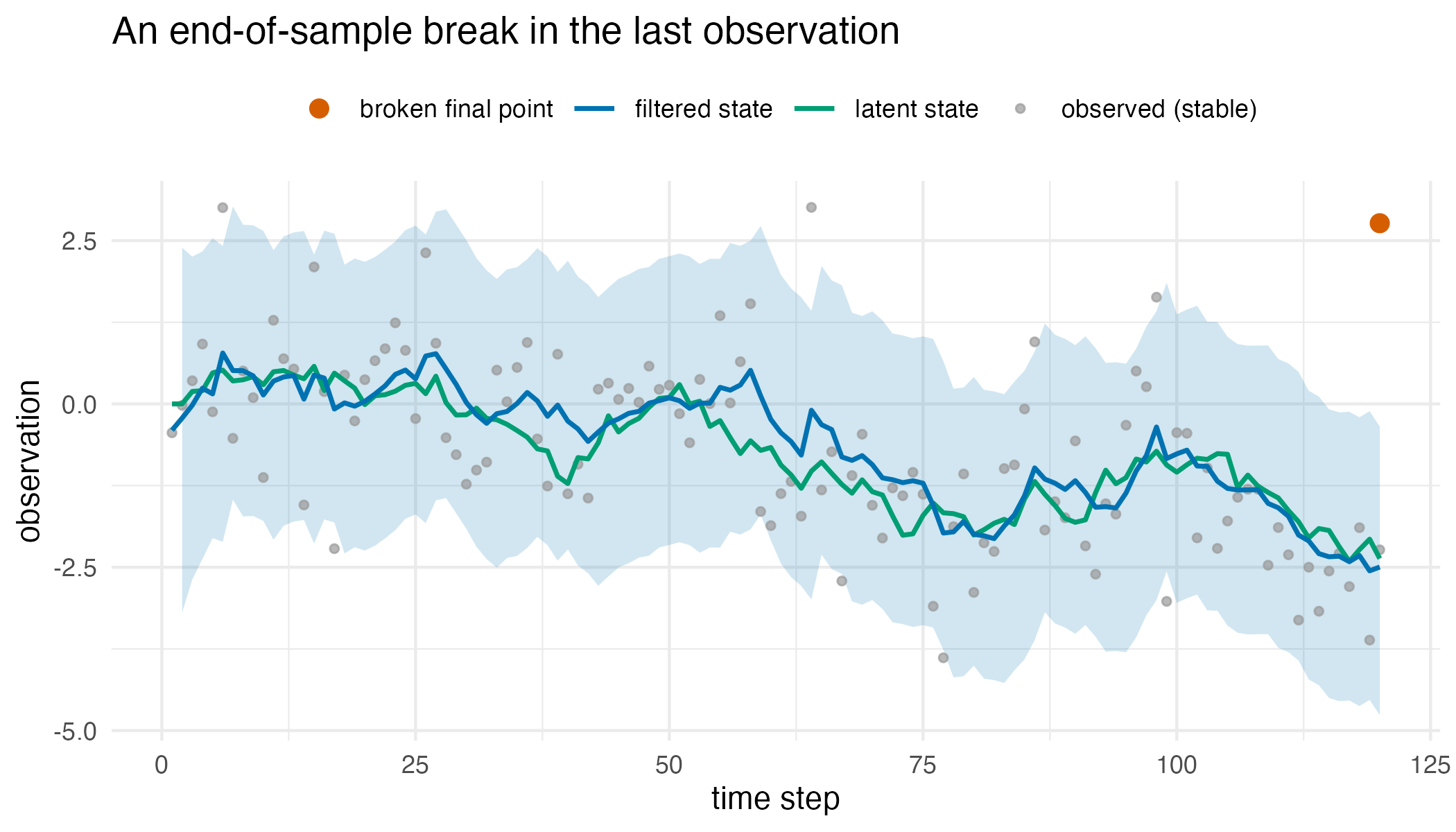

A time series of noisy observations in grey with the latent state and the filtered state overlaid and a shaded predictive band around the forecasts, and a single isolated point at the right-hand end sitting well above the band.

The local-level series, the latent state that generated it, the filtered state, and the one-step predictive band, two predictive standard deviations either side of the filter’s forecast of each observation. The band starts at the second step, after the diffuse prior. The broken final observation sits far outside the band, which is what inflates the statistic.

How the subsampling p-value is reached

The subsampling calibration compares the end-of-sample statistic with the in-sample blocks of the same series, so the p-value can be read straight off the empirical distribution of those blocks.

blocks_df <- rbind(
  data.frame(
    block = test_stable$in_sample_blocks, series = "stable series"
  ),
  data.frame(
    block = test_break$in_sample_blocks, series = "broken final point"
  )
)
blocks_df$series <- factor(
  blocks_df$series, levels = c("stable series", "broken final point")
)
rule_df <- data.frame(
  series = factor(
    c("stable series", "broken final point"),
    levels = c("stable series", "broken final point")
  ),
  statistic = c(test_stable$statistic, test_break$statistic)
)
ggplot2::ggplot(blocks_df, ggplot2::aes(block)) +
  ggplot2::stat_ecdf(geom = "step", linewidth = 0.8, colour = "#0072B2") +
  ggplot2::geom_vline(
    data = rule_df, ggplot2::aes(xintercept = statistic),
    colour = "#D55E00", linetype = "dashed", linewidth = 0.8
  ) +
  ggplot2::facet_wrap(~ series) +
  ggplot2::scale_x_log10(labels = function(v) {
    format(v, scientific = FALSE, drop0trailing = TRUE, trim = TRUE)
  }) +
  ggplot2::labs(
    x = "in-sample block statistic (log scale)",
    y = "cumulative share of blocks",
    title = "The end-of-sample statistic against its own in-sample blocks"
  ) +
  ggplot2::theme_minimal(base_size = 11)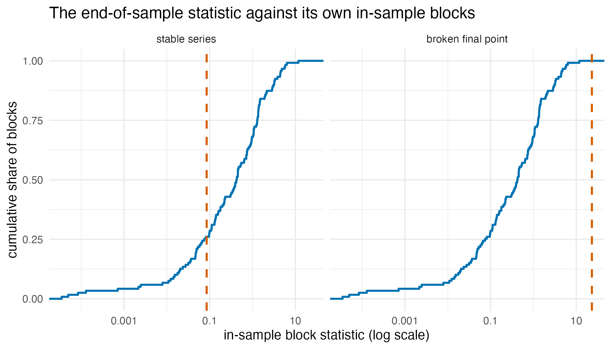

Two panels, each showing a rising step function of the cumulative share of in-sample block statistics against a logarithmic axis, annotated with a vertical rule; in the left panel the rule falls inside the curve, in the right panel it lies far beyond its right-hand end.

The empirical distribution of the in-sample block statistics for each series, with the end-of-sample statistic marked. The subsampling p-value is $(1 + k) / (n - 2m + 2)$ , where $k$ is the number of blocks lying at or beyond the dashed line, so the stable statistic sits inside the bulk while the broken one clears every block in the series.

What size the two calibrations actually hold

The chi-square calibration is exact when the model is given. The diffuse prior enters the forecast of the last observation with a weight that shrinks at every step, to about 0.0001 at $n = 30$ , so the chi-square reference is essentially exact here too. The size is still worth measuring rather than assuming. The study below simulates from the same local-level model under the null and records the rejection rate at a nominal 0.05, with the Monte Carlo standard error the replicate count supports.

simulate_null <- function(n_obs) {
  lv <- cumsum(c(0, rnorm(n_obs - 1L, 0, sqrt(0.04))))
  lv + rnorm(n_obs, 0, 1)
}
empirical_size <- function(n_obs, method, n_rep) {
  p <- vapply(seq_len(n_rep), function(i1) {
    gmm_eos_test(
      prior, dynamics, measurement, simulate_null(n_obs),
      m = 1L, method = method
    )$p_value
  }, numeric(1L))
  size <- mean(p < 0.05)
  c(size = size, se = sqrt(size * (1 - size) / n_rep), n_rep = n_rep)
} # ends empirical_size, one row of the size study

n_rep_short <- 250L
n_rep_long <- 150L
size_chisq_30 <- empirical_size(30L, "chisq", n_rep_short)
size_chisq_120 <- empirical_size(120L, "chisq", n_rep_long)
size_andrews_30 <- empirical_size(30L, "andrews", n_rep_short)

chisq_sizes <- c(size_chisq_30[["size"]], size_chisq_120[["size"]])
chisq_ses <- c(size_chisq_30[["se"]], size_chisq_120[["se"]])
chisq_worst_se <- max(abs(chisq_sizes - 0.05) / chisq_ses)

The subsampling p-value takes only the values $(1 + k) / (n - 2m + 2)$ for $k = 0, 1, \ldots$ . If the end block’s rank among the blocks is uniform, the size at a nominal level is the share of that grid below the level, and it can be computed without simulation. The rank is uniform when the blocks are exchangeable, which holds at $m = 1$ with the model given, apart from the first few innovations under the diffuse prior. It does not hold with estimated parameters, or for the overlapping blocks of $m > 1$ .

attainable_size <- function(n_obs, m = 1L, alpha = 0.05) {
  n_block <- n_obs - 2L * m + 1L
  p_grid <- (1L + seq.int(0L, n_block)) / (1L + n_block)
  mean(p_grid < alpha)
} # ends attainable_size, the size when the end block's rank is uniform

floor_30 <- 1 / (30L - 2L + 2L)
floor_120 <- 1 / (120L - 2L + 2L)
attainable_30 <- attainable_size(30L)
attainable_120 <- attainable_size(120L)
diff_30 <- size_chisq_30[["size"]] - size_andrews_30[["size"]]
diff_30_se <- sqrt(size_chisq_30[["se"]]^2 + size_andrews_30[["se"]]^2)
andrews_ses_from_grid <- abs(size_andrews_30[["size"]] - attainable_30) /
  size_andrews_30[["se"]]

Rejection rate against a nominal 0.05 under the null, simulated for both calibrations, and for the subsampling calibration also computed from its p-value grid, which gives its size when the end block’s rank is uniform. The grid values are not simulated, so their standard error and replicate cells hold a dash.
Calibration	n	Quantity	Value	Std. error	Replicates
chi-square	30	simulated size	0.0640	0.0155	250
chi-square	120	simulated size	0.0667	0.0204	150
subsampling	30	simulated size	0.0400	0.0124	250
subsampling	30	grid size, uniform rank	0.0333	–	–
subsampling	120	grid size, uniform rank	0.0417	–	–

Interpretation

On the stable series the statistic is 0.085 with a subsampling p-value of 0.742, and the test does not reject: the last observation sits where the filter expects it. Pushing that same observation five observation-noise standard deviations away lifts the statistic to 23.2, a p-value of 0.0083, and a rejection. That is the answer to the opening question in the form the analyst needs it: on this series, the arriving observation is flagged as inconsistent with the fitted model, and the same machinery leaves the unbroken series alone.

The first figure shows why. The broken point sits 4.8 predictive standard deviations from the filter’s forecast for $t = 120$ , the standardised innovation whose square is the statistic, far outside the band. Of the 119 stable observations from the second step on, 8 fall outside the band, or 6.7 per cent, against the 4.6 per cent a band of two standard deviations leaves out under the model. The second figure shows how that surprise becomes a p-value: for the stable series the statistic falls inside the bulk of the in-sample blocks, so a substantial share of blocks lie beyond it, while for the broken series it clears every one of the 119 blocks, which drives the p-value to its floor.

That floor is the first thing the size table makes concrete. At $n = 120$ and $m = 1$ the smallest attainable p-value is 0.0083, and the broken series attains it exactly. On a much shorter series the floor bites: at $n = 30$ the smallest attainable p-value is 0.033, so the subsampling calibration can reject at the 0.05 level only when the end-of-sample block is larger than every earlier block in the series. With the model given and $m = 1$ , the rank is uniform up to the first few innovations, so the size is the grid value: 0.0333 at $n = 30$ and 0.0417 at $n = 120$ , both below 0.05. The simulated size at $n = 30$ , 0.04 over 250 replicates with a standard error of 0.012, sits 0.5 standard errors from the grid value. With estimated parameters or $m > 1$ the grid value is not the size, and the simulation in the numerical illustration finds sizes above it.

The chi-square calibration is continuous and carries no such floor. Its simulated size is 0.064 at $n = 30$ (standard error 0.015, 250 replicates) and 0.067 at $n = 120$ (standard error 0.02, 150 replicates). Both sit within about 0.9 standard errors of the nominal 0.05, so at these replicate counts the study resolves no departure from nominal for either length. At $n = 30$ the simulated sizes of the two calibrations differ by 0.024, 1.2 standard errors of the difference, so the simulation does not resolve the contrast between them either. The contrast comes from the grid: with the model given, the subsampling test has a size of 0.0333 at $n = 30$ and $m = 1$ , while the chi-square calibration is continuous and can spend the full 0.05.

Limitations

A rejection rate estimated from 250 replicates carries a standard error near 0.014, so a departure from nominal of one or two percentage points is beyond the resolution of the size study above. It establishes the order of the size, not the exact size at a given series length.

The assumptions of both calibrations hold when the innovations are Gaussian. They part company when the observation noise is heavy-tailed: the parametric $\chi^2$ reference is then mis-specified, while the subsampling test judges the end-of-sample block only against the other blocks of the same series and needs no parametric reference. This vignette simulates Gaussian noise throughout and so does not exercise that divergence; method = "andrews" is the option to reach for when normality is in doubt, at the cost of the discreteness documented above. Which calibration is preferable therefore depends on which failure the analyst minds more: a mis-specified reference distribution, or a test that cannot spend its nominal level. The numerical illustration that follows places both calibrations beside the structural-break, changepoint and forecast-interval tools of four other packages, on the Nile series and in simulation.

The test is defined for a fitted linear-Gaussian state-space model, supplied exactly as for gmm_filter(): a single-component gmm prior, a dynamics list with the state-transition and process-noise matrices, and a measurement list with the observation and observation-noise matrices. Gaussian-sum process or measurement noise is rejected rather than approximated, because neither calibration is defined for it. The small-m regime (m = 1, 2, 3) is the point of the test, and m must be smaller than the series length.

One further caution belongs to the model rather than the test. The band in the first figure is the one-step predictive band, which the statistic divides by, not the filtered state’s standard deviation that gmm_filter() returns; at $t = 120$ the predictive standard deviation is 2.6 times the filtered one. A model whose noise covariances are themselves estimated on the same short series can understate both, and the test then inherits that optimism: it is a test of the last observation against the model, not a test of the model.

Numerical illustration

The Nile at 1898, with five packages

The annual flow of the Nile at Aswan, shipped with R as Nile, falls to a lower level after 1898 (Cobb, 1978). We fit a local-level model to the years 1871–1898 and ask each method whether the years that follow are consistent with it: 1899 alone, so $m = 1$ , and 1899–1901, so $m = 3$ . The documented change is the reference every method is scored against, and the score is a p-value at the 0.05 level.

Beside the two calibrations of gmm_eos_test() stand six tests: five from four packages and a t-test from base R. strucchange (Zeileis et al., 2002) supplies a sup-F test over the breaks whose final segment lies within the last $m$ years, and an OLS-based CUSUM test over the whole sample. changepoint (Killick and Eckley, 2014) supplies cpt.mean() with its defaults, the PELT search under the MBIC penalty, run on the series scaled to unit variance over the fitting years because its Normal cost takes the variance as one; it returns locations rather than a p-value, and a change located within the last $m$ years counts as a detection. KFAS (Helske, 2017) and dlm (Petris, 2010) each fit their own local level to 1871–1898 by maximum likelihood and check every tested year against its one-step forecast interval at level $1 - 0.05 / m$ , a Bonferroni correction. It would hold the check’s size at or below 0.05 whatever the window if the fitted parameters were the true ones; the simulation below measures the size with estimated parameters. The p-value reported is that of the largest standardised forecast error, times $m$ . The last test is a t-test on the residuals of the forecasts made at 1898 from the local level fitted by StructTS().

The four packages install from CRAN once and load as usual:

install.packages(c("strucchange", "changepoint", "KFAS", "dlm"))

library(strucchange)
library(changepoint)
library(KFAS)
library(dlm)

The fitting years are 1871–1898, and the local level is estimated on them alone:

nile <- as.numeric(window(Nile, 1871, 1901))
year <- 1871:1901
n_fit <- 28L
nile_fit <- nile[seq_len(n_fit)]

level_fit <- StructTS(nile_fit, type = "level")
prior_nile <- gmm(weights = 1, means = list(nile_fit[1L]),
                  covariances = list(matrix(1e7)))
dynamics_nile <- list(A = matrix(1), Q = matrix(level_fit$coef[["level"]]))
measurement_nile <- list(C = matrix(1),
                         R = matrix(level_fit$coef[["epsilon"]]))

The state-space fits and the t-test use those years alone and are applied to the series truncated $m$ years later; the strucchange tests and cpt.mean() run on the whole truncated series. A test that is not defined at that window returns NA, which the table below prints as “not defined”.

nile_tests <- function(m) {
  y <- nile[seq_len(n_fit + m)]
  n <- length(y)
  last <- (n_fit + 1L):n

  p_chisq <- gmm_eos_test(prior_nile, dynamics_nile, measurement_nile, y,
                          m = m, method = "chisq")$p_value
  p_andrews <- gmm_eos_test(prior_nile, dynamics_nile, measurement_nile, y,
                            m = m, method = "andrews")$p_value

  # strucchange needs at least two observations after a break in a mean
  p_supf <- if (m >= 2L) {
    unname(sctest(Fstats(y ~ 1, from = n - m, to = n - 2L))$p.value)
  } else NA_real_
  p_cusum <- unname(sctest(efp(y ~ 1, type = "OLS-CUSUM"))$p.value)

  cp <- cpts(cpt.mean(y / sd(nile_fit)))
  found_cpt <- any(cp >= n_fit)

  kfas_fit <- fitSSM(SSModel(nile_fit ~ SSMtrend(1L, Q = NA), H = NA),
                     inits = log(c(var(nile_fit), var(nile_fit))),
                     method = "BFGS")
  kfas_model <- SSModel(y ~ SSMtrend(1L, Q = kfas_fit$model$Q[1L]),
                        H = kfas_fit$model$H[1L])
  kfas_pred <- predict(kfas_model, interval = "prediction", level = 0.95,
                       filtered = TRUE)
  kfas_z <- (y[last] - kfas_pred[last, "fit"]) /
    ((kfas_pred[last, "upr"] - kfas_pred[last, "lwr"]) / (2 * qnorm(0.975)))
  p_kfas <- min(1, m * 2 * pnorm(-max(abs(kfas_z))))

  dlm_build <- function(pars) {
    dlmModPoly(1L, dV = exp(pars[1L]), dW = exp(pars[2L]))
  }
  dlm_fit <- dlmMLE(nile_fit, parm = log(c(var(nile_fit), var(nile_fit))),
                    build = dlm_build)
  dlm_filt <- dlmFilter(y, dlm_build(dlm_fit$par))
  dlm_var <- unlist(dlmSvd2var(dlm_filt$U.R, dlm_filt$D.R)) +
    exp(dlm_fit$par[1L])
  dlm_z <- (y[last] - dlm_filt$f[last]) / sqrt(dlm_var[last])
  p_dlm <- min(1, m * 2 * pnorm(-max(abs(dlm_z))))

  resid <- y[last] - predict(level_fit, n.ahead = m)$pred
  p_t <- if (m > 1L) t.test(resid)$p.value else NA_real_

  list(
    p = c("proxymix chi-square" = p_chisq,
          "proxymix subsampling" = p_andrews,
          "strucchange sup-F" = p_supf,
          "strucchange OLS-CUSUM" = p_cusum,
          "KFAS forecast interval" = p_kfas,
          "dlm forecast interval" = p_dlm,
          "t-test on forecast residuals" = p_t),
    found_cpt = found_cpt
  )
}

nile_1 <- nile_tests(1L)
nile_3 <- nile_tests(3L)

Each test’s p-value on the Nile series fitted to 1871–1898, for 1899 (m = 1) and for 1899–1901 (m = 3), against the documented change at 1898; cpt.mean reports a location rather than a p-value.
Test	m = 1	m = 3
proxymix chi-square	0.018 (reject)	0.012 (reject)
proxymix subsampling	0.034 (reject)	0.037 (reject)
strucchange sup-F	not defined	0.003 (reject)
strucchange OLS-CUSUM	0.881	0.427
KFAS forecast interval	0.018 (reject)	0.055
dlm forecast interval	0.018 (reject)	0.055
t-test on forecast residuals	not defined	0.012 (reject)
changepoint cpt.mean	no change located	no change located

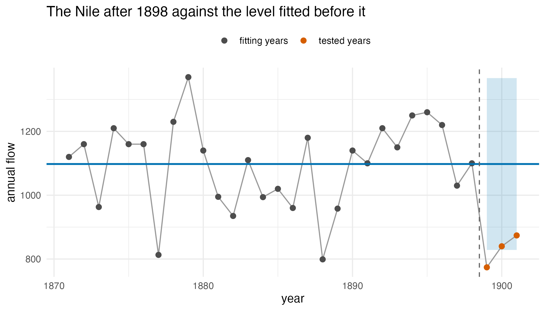
A line of annual Nile flows from 1871 to 1901, a horizontal fitted level through 1898 with a shaded forecast band extending over 1899 to 1901, and the 1899 to 1901 points lying at or below the lower edge of the band.

The Nile flow for 1871–1901 with the local level fitted to 1871–1898 and its 95% forecast band for the three years that follow. The dashed vertical line separates the fitting years from the tested years. The 1899 observation falls below the band.

The local level fitted to 1871–1898 has a level variance of zero, so the model is a constant mean with an observation standard deviation of 135, and the 1899 flow sits 2.40 of those standard deviations below it. At $m = 1$ the chi-square calibration returns a p-value of 0.018, and the KFAS and dlm interval checks return 0.018 and 0.018: at a single observation the three are the same test, a one-step forecast error referred to its standard deviation, and they differ only in the fitted variances. The subsampling calibration returns 0.034, which is its floor of $1 / (n - 2m + 2) = 1 / 29$ at this length: the 1899 block is the largest in the series. The sup-F test is not defined at $m = 1$ , because strucchange’s Fstats() admits a break in a mean no later than $n - 2$ , so at least two observations must follow it. The t-test is not defined at $m = 1$ either, because it estimates the variance of the forecast residuals from the tested years themselves. Chow’s predictive test, which takes that variance from the fitting years, is defined at one observation. The OLS-CUSUM test, which asks about the whole sample, returns 0.881. cpt.mean() locates no change on the scaled series. At $m = 3$ the sup-F test is defined and returns 0.003, the chi-square calibration 0.012 and the t-test 0.012, while the interval checks, spending their level over three years, return 0.055 and 0.055. The subsampling p-value is again at its floor, $1 / 27$ . This is one series and one documented change, which shows which tests exist at each window but cannot measure their size or power, so the simulation below does.

A simulation benchmark

The simulation generates 1000 stationary AR(1) series of length 100 with coefficient 0.6 and unit innovation variance. For each series and each window $m \in \{1, 3, 5\}$ , every method is applied twice: to the series as generated, which gives the size, and to the series with its last $m$ observations raised by 3 innovation standard deviations, which gives the power. The state-space methods and the t-test are fitted to the first $n - m$ observations; the strucchange tests and cpt.mean() run on the whole series, as described below. The reference is the design itself, whether or not a shift was applied, and the score is the rejection rate at a nominal 0.05.

proxymix and the t-test receive the AR(1) fitted by arima(), written as a state-space model with the state observed exactly; the t-test’s residuals are those of the forecasts made at $n - m$ . KFAS and dlm each fit their own AR(1) to the fitting window after its mean is removed, and check the last $m$ observations against one-step forecast intervals at level $1 - 0.05 / m$ , as on the Nile. strucchange runs the sup-F test on the regression of $y_t$ on $y_{t-1}$ over the breaks whose final segment lies within the last $m$ observations, which needs at least three observations after the break, so it is defined at $m = 3$ and $m = 5$ and not at $m = 1$ . Its OLS-CUSUM test runs over the whole sample. cpt.mean() runs on the series scaled to unit variance over the fitting window, and a change located within the last $m$ observations counts as a rejection. A rejection rate near 0.05 from 1000 series carries a Monte Carlo standard error of about 0.007, and one near 0.5 about 0.016. This chunk is complete and runs as shown, but it took about 18 minutes on one core (R 4.6.1, Apple silicon), so the table that follows it is read from its stored output. For a quick reduced run, set n_rep to a small number such as 20L on the line that defines it.

library(proxymix)
library(strucchange)
library(changepoint)
library(KFAS)
library(dlm)

n <- 100L        # length of each series
phi <- 0.6       # autoregressive coefficient
delta <- 3       # level shift, in innovation standard deviations
m_vec <- c(1L, 3L, 5L)
n_rep <- 1000L   # series per window

# every test is fitted to the first n - m observations of y and applied to
# its last m; NA marks a test that is not defined at that window
p_values <- function(y, m) {
  n <- length(y)
  y_fit <- y[seq_len(n - m)]
  last <- (n - m + 1L):n

  ar <- arima(y_fit, order = c(1L, 0L, 0L))
  a1 <- coef(ar)[["ar1"]]
  mu <- coef(ar)[["intercept"]]
  s2 <- ar$sigma2
  prior <- gmm(weights = 1, means = list(mu),
               covariances = list(matrix(s2 / (1 - a1^2))))
  dynamics <- list(A = matrix(a1), b = mu * (1 - a1), Q = matrix(s2))
  measurement <- list(C = matrix(1), R = matrix(0))
  p_chisq <- gmm_eos_test(prior, dynamics, measurement, y, m = m,
                          method = "chisq")$p_value
  p_andrews <- gmm_eos_test(prior, dynamics, measurement, y, m = m,
                            method = "andrews")$p_value
  resid <- y[last] - predict(ar, n.ahead = m)$pred
  p_t <- if (m > 1L) t.test(resid)$p.value else NA_real_

  # strucchange needs at least three observations after a break in an AR(1)
  reg <- data.frame(y = y[-1L], y_lag = y[-n])
  n_reg <- nrow(reg)
  p_supf <- if (m >= 3L) {
    fs <- Fstats(y ~ y_lag, data = reg, from = n_reg - m, to = n_reg - 3L)
    unname(sctest(fs)$p.value)
  } else NA_real_
  p_cusum <- unname(sctest(efp(y ~ y_lag, data = reg,
                               type = "OLS-CUSUM"))$p.value)

  cp <- cpts(cpt.mean(y / sd(y_fit)))
  p_cpt <- if (any(cp >= n - m)) 0 else 1

  y_bar <- mean(y_fit)
  kfas_update <- function(pars, model) {
    part <- SSMarima(ar = 0.999 * tanh(pars[1L]), Q = exp(pars[2L]))
    model["T", "arima"] <- part$T
    model["R", "arima"] <- part$R
    model["Q", "arima"] <- part$Q
    model["P1", "arima"] <- part$P1
    model
  }
  kfas_fit <- fitSSM(
    SSModel(I(y_fit - y_bar) ~ -1 + SSMarima(ar = 0.5, Q = 1), H = 0),
    inits = c(0, 0), updatefn = kfas_update, method = "BFGS"
  )
  kfas_par <- kfas_fit$optim.out$par
  kfas_model <- SSModel(
    I(y - y_bar) ~ -1 + SSMarima(ar = 0.999 * tanh(kfas_par[1L]),
                                  Q = exp(kfas_par[2L])),
    H = 0
  )
  kfas_pred <- predict(kfas_model, interval = "prediction", level = 0.95,
                       filtered = TRUE)
  kfas_z <- (y[last] - y_bar - kfas_pred[last, "fit"]) /
    ((kfas_pred[last, "upr"] - kfas_pred[last, "lwr"]) / (2 * qnorm(0.975)))
  p_kfas <- min(1, m * 2 * pnorm(-max(abs(kfas_z))))

  dlm_build <- function(pars) {
    dlmModARMA(ar = 0.999 * tanh(pars[1L]), sigma2 = exp(pars[2L]), dV = 0)
  }
  dlm_fit <- dlmMLE(y_fit - y_bar, parm = c(0, 0), build = dlm_build)
  dlm_filt <- dlmFilter(y - y_bar, dlm_build(dlm_fit$par))
  dlm_var <- unlist(dlmSvd2var(dlm_filt$U.R, dlm_filt$D.R))
  dlm_z <- (y[last] - y_bar - dlm_filt$f[last]) / sqrt(dlm_var[last])
  p_dlm <- min(1, m * 2 * pnorm(-max(abs(dlm_z))))

  c("proxymix chi-square" = p_chisq, "proxymix subsampling" = p_andrews,
    "strucchange sup-F" = p_supf, "strucchange OLS-CUSUM" = p_cusum,
    "changepoint cpt.mean" = p_cpt, "KFAS forecast interval" = p_kfas,
    "dlm forecast interval" = p_dlm, "t-test on forecast residuals" = p_t)
}

one_series <- function(r) {
  set.seed(r)
  y <- as.numeric(arima.sim(list(ar = phi), n = n))
  do.call(rbind, lapply(m_vec, function(m) {
    y_shift <- y
    y_shift[(n - m + 1L):n] <- y_shift[(n - m + 1L):n] + delta
    p_null <- p_values(y, m)
    p_shift <- p_values(y_shift, m)
    data.frame(r = r, m = m, method = rep(names(p_null), 2L),
               scenario = rep(c("no shift", "shift"), each = length(p_null)),
               reject = c(p_null, p_shift) < 0.05,
               stringsAsFactors = FALSE)
  }))
}

res <- do.call(rbind, lapply(seq_len(n_rep), one_series))

sim_tab <- aggregate(reject ~ m + scenario + method, data = res, FUN = mean,
                     na.action = na.pass)
names(sim_tab)[4L] <- "rate"
sim_tab$se <- sqrt(sim_tab$rate * (1 - sim_tab$rate) / n_rep)
sim_tab

Rejection rate at a nominal 0.05 over 1000 simulated AR(1) series per window: the size, without a shift, and the power, with the last m observations raised by 3 innovation standard deviations, scored against the design. The number in each column heading is the window m. A dash marks a test that is not defined at that window.
Test	Size 1	Power 1	Size 3	Power 3	Size 5	Power 5
proxymix chi-square	0.068	0.834	0.064	0.835	0.070	0.852
proxymix subsampling	0.049	0.798	0.062	0.801	0.073	0.830
strucchange sup-F	–	–	0.237	0.972	0.038	0.810
strucchange OLS-CUSUM	0.018	0.021	0.018	0.014	0.018	0.014
changepoint cpt.mean	0.001	0.088	0.007	0.461	0.018	0.645
KFAS forecast interval	0.090	0.836	0.094	0.777	0.090	0.777
dlm forecast interval	0.069	0.830	0.070	0.772	0.070	0.782
t-test on forecast residuals	–	–	0.146	0.777	0.269	0.972

Of the eight tests, six are defined at $m = 1$ . Four of them score the one-step forecast error of the last observation: the two calibrations of gmm_eos_test() and the forecast-interval checks of KFAS and dlm, which at one observation are the same statistic as the chi-square calibration, with parameters from each package’s own fit. The powers of the chi-square calibration, KFAS and dlm are within 0.006 of each other, at 0.834 for the chi-square calibration, 0.836 for KFAS and 0.830 for dlm, and their sizes are 0.068, 0.090 and 0.069, all above the nominal 0.05, because the parameters are estimated on the fitting window and the tests treat them as known. The subsampling rank does not depend on the innovation variance, which scales every block alike, but it still uses the estimated autoregressive coefficient and mean, and its in-sample blocks are residuals of the fit while the end block is not. It has a size of 0.049 and a power of 0.798 at $m = 1$ . The sup-F test and the t-test are not defined, the OLS-CUSUM test rejects the shifted series in 0.021 of cases, and cpt.mean() locates a change in the last observation in 0.088 of shifted series against 0.001 of unshifted ones.

Across the three windows the chi-square calibration’s size is 0.064 to 0.070 and its power 0.834 to 0.852; the subsampling calibration’s size is 0.049 to 0.073 and its power 0.798 to 0.830. The interval checks keep their size near its $m = 1$ value, with KFAS at 0.090 to 0.094 and dlm at 0.069 to 0.070. Their power falls from 0.836 at $m = 1$ to 0.777 at $m = 3$ for KFAS and from 0.830 to 0.772 for dlm, because each check’s level is divided by $m$ and under an AR(1) only the first shifted observation carries the whole shift in its one-step forecast error, the later ones carry $1 - \phi$ of it. The sup-F test at $m = 3$ has one admissible break and rejects 0.237 of unshifted series with strucchange 1.6-0, because its p-value comes from an asymptotic approximation for a break range that this window places at the edge of the sample; at $m = 5$ its size is 0.038 and its power 0.810, against 0.852 at a size of 0.070 for the chi-square calibration. The t-test on the forecast residuals rejects 0.146 and 0.269 of unshifted series at $m = 3$ and $m = 5$ , because the residuals of forecasts made at one origin are correlated and the test takes them as independent. The OLS-CUSUM test rejects unshifted series at a rate of 0.018 at every window and shifted ones at 0.014 to 0.021; a shift confined to the last few observations barely moves a cumulative sum over the whole sample. cpt.mean() locates a change in the last $m$ observations of unshifted series at a rate of 0.001 to 0.018 and of shifted ones at 0.088 to 0.645. A size estimated from 1000 series has a Monte Carlo standard error of about 0.007, so the sizes of the chi-square calibration and of the interval checks sit 2.0 to 6.4 standard errors above 0.05, and the subsampling size at $m = 1$ is not distinguished from it.

In this run the subsampling calibration of gmm_eos_test() was the only one of the six tests defined at $m = 1$ to hold a size within a standard error of nominal there, with a power of 0.798. At $m = 3$ and $m = 5$ its size was 0.062 and 0.073, 1.7 and 3.3 standard errors above 0.05. Its grid values at $n = 100$ are 0.040, 0.042 and 0.043 at $m = 1$ , 3 and 5, which are the size only when the end block’s rank is uniform; with estimated parameters and overlapping blocks it is not. At $m = 5$ the sup-F test of strucchange had a size closer to nominal than either calibration, 0.038, and a power of 0.810 against 0.852 for the chi-square calibration and 0.830 for the subsampling calibration. The t-test had the highest rejection rate under the shift at $m = 5$ , 0.972, and 0.777 at $m = 3$ against 0.972 for the sup-F test, but its size was 2.9 and 5.4 times the nominal level at $m = 3$ and $m = 5$ , so these rates are not comparable to the powers of tests that hold their size. The comparison covers one autoregressive coefficient, one series length, one shift size and a level shift confined to the tested window, not the smaller or gradual shifts, the longer windows, or the non-Gaussian innovations under which the two calibrations part company.

References

Andrews, D. W. K. (1993). Tests for parameter instability and structural change with unknown change point. Econometrica 61(4), 821–856. https://doi.org/10.2307/2951764.
Andrews, D. W. K. (2003). End-of-sample instability tests. Econometrica 71(6), 1661–1694. https://doi.org/10.1111/1468-0262.00466.
Chow, G. C. (1960). Tests of equality between sets of coefficients in two linear regressions. Econometrica 28(3), 591–605. https://doi.org/10.2307/1910133.
Cobb, G. W. (1978). The problem of the Nile: conditional solution to a changepoint problem. Biometrika 65(2), 243–251. https://doi.org/10.1093/biomet/65.2.243.
Helske, J. (2017). KFAS: Exponential family state space models in R. Journal of Statistical Software 78(10), 1–39. https://doi.org/10.18637/jss.v078.i10.
Killick, R. and Eckley, I. A. (2014). changepoint: An R package for changepoint analysis. Journal of Statistical Software 58(3), 1–19. https://doi.org/10.18637/jss.v058.i03.
Petris, G. (2010). An R package for dynamic linear models. Journal of Statistical Software 36(12), 1–16. https://doi.org/10.18637/jss.v036.i12.
Zeileis, A., Leisch, F., Hornik, K. and Kleiber, C. (2002). strucchange: An R package for testing for structural change in linear regression models. Journal of Statistical Software 7(2), 1–38. https://doi.org/10.18637/jss.v007.i02.

Reproduce

The vignette sets set.seed(20260621) once, before the series is simulated, and every result up to the numerical illustration – the two tests, the filter path and both size studies – is a deterministic function of that stream.

The Nile illustration draws nothing at random: every fit is a maximum likelihood estimate from fixed starting values. In the simulation each series is generated after set.seed() with its own index, and both scenarios at every window share that series. The stored simulation results come from the code shown, run on 26 September 2026 with R 4.6.1, proxymix 0.16.0, strucchange 1.6-0, changepoint 2.3, KFAS 1.6.0 and dlm 1.1-6.1, and the run raised 0 warnings.

print(sessionInfo(), locale = FALSE)

#> R version 4.6.1 (2026-06-24)
#> Platform: aarch64-apple-darwin23
#> Running under: macOS Tahoe 26.6.2
#> 
#> Matrix products: default
#> BLAS:   /Library/Frameworks/R.framework/Versions/4.6/Resources/lib/
#>     libRblas.0.dylib 
#> LAPACK: /Library/Frameworks/R.framework/Versions/4.6/Resources/lib/
#>     libRlapack.dylib;  LAPACK version 3.12.1
#> 
#> attached base packages:
#> [1] stats     graphics  grDevices utils     datasets  methods  
#> [7] base     
#> 
#> other attached packages:
#> [1] dlm_1.1-6.1       KFAS_1.6.0        changepoint_2.3  
#> [4] strucchange_1.6-0 sandwich_3.1-3    zoo_1.9-0        
#> [7] proxymix_0.16.0  
#> 
#> loaded via a namespace (and not attached):
#>  [1] mvnfast_0.2.8      gtable_0.3.6       jsonlite_2.0.0    
#>  [4] dplyr_1.2.1        compiler_4.6.1     Rcpp_1.1.2        
#>  [7] tidyselect_1.2.1   dichromat_2.0-1    jquerylib_0.1.4   
#> [10] systemfonts_1.3.2  scales_1.4.0       textshaping_1.0.5 
#> [13] yaml_2.3.12        fastmap_1.2.0      lattice_0.23-1    
#> [16] ggplot2_4.0.3      R6_2.6.1           labeling_0.4.3    
#> [19] generics_0.1.4     knitr_1.51         htmlwidgets_1.6.4 
#> [22] tibble_3.3.1       desc_1.4.3         bslib_0.12.0      
#> [25] pillar_1.11.1      RColorBrewer_1.1-3 rlang_1.3.0       
#> [28] cachem_1.1.0       xfun_0.60          fs_2.1.0          
#> [31] sass_0.4.10        S7_0.2.2           otel_0.2.0        
#> [34] cli_3.6.6          withr_3.0.3        pkgdown_2.2.1     
#> [37] magrittr_2.0.5     digest_0.6.39      grid_4.6.1        
#> [40] lifecycle_1.0.5    vctrs_0.7.3        evaluate_1.0.5    
#> [43] glue_1.8.1         farver_2.1.2       ragg_1.5.2        
#> [46] rmarkdown_2.32     tools_4.6.1        pkgconfig_2.0.3   
#> [49] htmltools_0.5.9