From KDE: compressing a kernel density estimate into a Gaussian-mixture proxy

library(proxymix)
library(ggplot2)

Why a `from_kde()` constructor

A kernel density estimate (KDE) gives a smooth, non-parametric density from a sample of n points, but with three operational costs:

No closed-form marginals. Integrating out a coordinate of a KDE requires a numerical sweep over the kernel mixture.
No closed-form conditioning. There is no analogue of the Schur complement; one has to resample or build a conditional KDE per query.
No native aggregation algebra. Pushforwards through linear operators, observation-channel updates, or block-sums all collapse to Monte Carlo.

proxymix::from_kde() compresses the KDE into an N-component Gaussian mixture proxy (with N typically much smaller than n) by treating the KDE as a normalised, evaluable target and running regime (iii) KLD-EM against it. The proxy then supports the full closed-form operator set exposed by the rest of the package – dgmm(), rgmm(), gmm_marginalise(), gmm_conditionalise(), plus the v0.3 affine-Gaussian calculus (gmm_affine(), gmm_observe()).

This is not new science. It is a practical bridge between a non-parametric density estimate and a parametric closed-form mixture representation. The bias inherited from the KDE is reproduced in the proxy; the bandwidth controls the bias-variance trade-off.

Recovering a known mixture

Sample from a known bimodal mixture and ask from_kde() to recover it.

set.seed(1L)
true_means <- list(c(-2, 0), c(2, 0))
true_cov   <- diag(2)
x <- rbind(
  mvnfast::rmvn(150L, mu = true_means[[1L]], sigma = true_cov),
  mvnfast::rmvn(150L, mu = true_means[[2L]], sigma = true_cov)
)

fit <- from_kde(
  x, N = 2L,
  bandwidth = "silverman",
  is_size = 2000L, max_iter = 60L, seed = 1L,
  validation_size = 2000L
)
fit
#> <gmm_fit>: regime = "kld", K = 2, p = 2
#>   target     : from_kde
#>   iterations : 15
#>   converged  : TRUE
#>   [1] w = 0.5083, |mu| = 1.9840, tr(Sigma) = 3.0490
#>   [2] w = 0.4917, |mu| = 2.2039, tr(Sigma) = 2.4588

The proxy components sit near the true means.

vapply(fit@means, function(mu) round(mu, 2L), numeric(2L))
#>       [,1]  [,2]
#> [1,] -1.98  2.20
#> [2,]  0.05 -0.08

Quality of the importance-sampled fit

Inspect ESS and the largest self-normalised weight: a healthy regime-(iii) fit has ESS close to is_size and a max-weight share of a few percent.

ess_summary(fit)
#> $is_size
#> [1] 2000
#> 
#> $ess
#> [1] 1532.381
#> 
#> $ess_relative
#> [1] 0.7661903
#> 
#> $max_weight
#> [1] 0.001171959
#> 
#> $support_fraction
#> [1] 1
#> 
#> $mc_se_kld
#> [1] 0.005589403
#> 
#> $validation_size
#> [1] 2000
#> 
#> $validation_ess
#> [1] 1530.978
#> 
#> $validation_ess_relative
#> [1] 0.7654892
#> 
#> $validation_max_weight
#> [1] 0.00116206
#> 
#> $validation_support_fraction
#> [1] 1
#> 
#> $validation_kld
#> [1] 0.02483515

The validation block reports a held-out KLD on an independent IS draw – a safeguard against in-sample overfitting to one particular IS realisation.

Bandwidth sensitivity

Smaller bandwidths track the data more tightly (lower bias, higher variance); larger bandwidths smooth the proxy. The proxy inherits this trade-off.

bandwidth_grid <- c(0.2, 0.5, 1.0)
fits <- lapply(bandwidth_grid, function(h) {
  from_kde(x, N = 2L, bandwidth = h,
           is_size = 1500L, max_iter = 40L, seed = 1L)
})

data.frame(
  bandwidth      = bandwidth_grid,
  ess            = vapply(fits, function(f) f@diagnostics$ess, numeric(1L)),
  max_weight     = vapply(fits, function(f) f@diagnostics$max_weight, numeric(1L)),
  trace_Sigma_k1 = vapply(fits, function(f) sum(diag(f@covariances[[1L]])), numeric(1L))
)
#>   bandwidth       ess  max_weight trace_Sigma_k1
#> 1       0.2  768.4537 0.007158846       2.165142
#> 2       0.5  997.8578 0.001887074       2.463437
#> 3       1.0 1189.3327 0.001287610       3.816308

Visualising the compression

Compare the KDE log-density and the proxy log-density on a planar grid.

grid <- expand.grid(
  x = seq(-5, 5, length.out = 80L),
  y = seq(-4, 4, length.out = 60L)
)
gm <- as.matrix(grid)
kde_log_density <- fit@target@log_density
grid$kde   <- kde_log_density(gm)
grid$proxy <- log(dgmm(gm, fit))

## Shared contour levels so the two log-densities are directly comparable.
brks <- pretty(range(c(grid$kde, grid$proxy), finite = TRUE), 9L)
ggplot() +
  geom_point(data = as.data.frame(x), aes(V1, V2),
             colour = "grey55", alpha = 0.25, size = 0.5) +
  geom_contour(data = grid,
               aes(x, y, z = kde, colour = "KDE", linetype = "KDE"),
               breaks = brks, linewidth = 0.45) +
  geom_contour(data = grid,
               aes(x, y, z = proxy,
                   colour = "Mixture proxy", linetype = "Mixture proxy"),
               breaks = brks, linewidth = 0.55) +
  scale_colour_manual(name = NULL,
                      values = c("KDE" = "#2C7FB8",
                                 "Mixture proxy" = "#D95F0E")) +
  scale_linetype_manual(name = NULL,
                        values = c("KDE" = "solid",
                                   "Mixture proxy" = "dashed")) +
  coord_equal(expand = FALSE) +
  labs(title = "KDE and Gaussian-mixture proxy (log-density contours)",
       x = expression(x[1]), y = expression(x[2])) +
  theme_minimal(base_size = 11) +
  theme(plot.title = element_text(face = "bold"),
        legend.position = "top",
        panel.grid.minor = element_blank())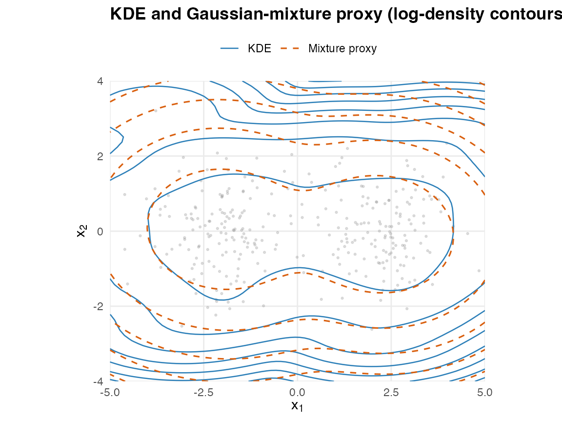

Scope and limits (v0.2)

Dimensional cap. from_kde() is well-tested for p <= 5; it warns between p = 6 and p = 10, and refuses p > 10. Regime (iii) is driven by importance sampling, whose effective sample size falls sharply in high dimensions. For richer ambient spaces, compose a low-p proxy with the affine-Gaussian operator calculus rather than fitting in the ambient space.
Bandwidth shapes. Only scalar and diagonal bandwidths are supported. A full-matrix bandwidth effectively encodes a covariance estimate and blurs the KDE-vs-mixture distinction; if that is what you want, fit the mixture directly with fit_proxymix(regime = "sample").
Normalisation. A KDE is normalised by construction, so the returned gmm_target declares normalised = TRUE and log_normalizer = 0. This makes hellinger_mc() meaningful and lets the KLD diagnostics report absolute values, not shifted ones.
What this is not. It is not a method for picking the KDE bandwidth. Use the conventional rules of thumb ("silverman", "scott") or a cross-validation procedure outside the package, then pass the chosen bandwidth in.

When to prefer `fit_proxymix(regime = "sample")` instead

If your goal is “find a Gaussian-mixture density given samples”, the classical EM regime is more direct, fits in linear time, and does not incur the regime-(iii) importance-sampling tax. from_kde() only earns its place when you specifically want the KDE’s smoothing as a step in your pipeline – e.g. as part of a sequence such as

samples |> from_kde() |> gmm_conditionalise() |> rgmm()

– or when the KDE’s bias-variance trade-off is part of what you are trying to validate downstream.

References

Hoek, J. van der and Elliott, R. J. (2024). Mixtures of multivariate Gaussians. Stochastic Analysis and Applications. doi:10.1080/07362994.2024.2372605.
Silverman, B. W. (1986). Density Estimation for Statistics and Data Analysis. CRC Press.
Scott, D. W. (1992). Multivariate Density Estimation: Theory, Practice, and Visualization. Wiley.

Why a from_kde() constructor