This vignette walks through the three KL-optimal regimes of Hoek and Elliott (2024). For each, we show what information the regime needs about the target, the M-step update it implements, and an end-to-end fit on a target whose ground truth we know.
We use the bundled three-component mixture target – its log-density is known exactly, and (because the target is itself a Gaussian mixture) so are its true samples.
tgt <- mixture_target(with_samples = TRUE, n = 1500L, seed = 1L)
tgt
#> <gmm_target>: "three_mixture" in p = 2 dimensions
#>   log_density : supplied
#>   samples     : 1500 x 2 matrix
#>   normalised  : TRUE
#>   log Z(f)    : 0
if (requireNamespace("ggplot2", quietly = TRUE)) {
  library(ggplot2)
  grid_x <- seq(-4.5, 4.5, length.out = 100)
  G <- expand.grid(x1 = grid_x, x2 = grid_x)
  G$f <- exp(tgt@log_density(as.matrix(G)))
  ggplot(G, aes(x1, x2)) +
    geom_contour_filled(aes(z = f), bins = 10L, alpha = 0.9) +
    geom_point(data = as.data.frame(tgt@samples[1:500, ]),
               aes(V1, V2), alpha = 0.15, size = 0.6) +
    scale_fill_viridis_d(option = "mako", guide = "none") +
    coord_equal() +
    labs(x = expression(x[1]), y = expression(x[2])) +
    theme_minimal(base_size = 12)
}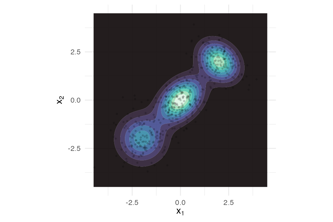
Three-mixture target with overlaid samples.
Regime (i): closed-form moment matching
When N == 1, the KL-optimal Gaussian proxy has the same
mean and covariance as the target. That is regime (i). The function is
fit_moment_match(), and the dispatcher chooses it under
regime = "auto" when N == 1 and samples (or
moments) are available.
m_fit <- fit_proxymix(tgt, N = 1L, regime = "moment")
m_fit
#> <gmm_fit>: regime = "moment", K = 1, p = 2
#>   target     : three_mixture
#>   iterations : 0
#>   converged  : TRUE
#>   [1] w = 1.0000, |mu| = 0.0328, tr(Sigma) = 5.6029
Recovered mean and covariance match the target’s empirical moments to within sampling error:
m_fit@means[[1L]]
#> [1] -0.01240519 -0.03037255
m_fit@covariances[[1L]]
#>          [,1]     [,2]
#> [1,] 2.731676 2.332994
#> [2,] 2.332994 2.871190
A single Gaussian is, of course, a bad fit to a three-mode mixture –
but it is the KL-optimal single Gaussian. Regime (i) is most
useful when used as a deterministic seed for regimes (ii) or
(iii) at N > 1.
Regime (ii): classical EM on samples
When the target carries samples, the textbook EM algorithm fits an
N-component Gaussian mixture by maximum likelihood. That is
regime (ii). The algorithm is the standard
iterate-until-convergence:
- E-step – .
-
M-step – re-weight
by the responsibilities, with a diagonal ridge
epsilon_covto keep positive-definite. -
Convergence – relative change in the empirical
log-likelihood below
tol.
s_fit <- fit_proxymix(tgt, N = 3L, regime = "sample",
                      max_iter = 200L, n_starts = 4L)
s_fit
#> <gmm_fit>: regime = "sample", K = 3, p = 2
#>   target     : three_mixture
#>   iterations : 53
#>   converged  : TRUE
#>   [1] w = 0.4074, |mu| = 0.0335, tr(Sigma) = 0.9418
#>   [2] w = 0.3025, |mu| = 2.7614, tr(Sigma) = 1.2135
#>   [3] w = 0.2901, |mu| = 2.8208, tr(Sigma) = 0.8067
The log-likelihood trace is monotone-up:
trace <- s_fit@diagnostics$loglik_trace
if (requireNamespace("ggplot2", quietly = TRUE)) {
  ggplot(data.frame(iter = seq_along(trace), loglik = trace),
         aes(iter, loglik)) +
    geom_line() + geom_point(size = 1) +
    labs(x = "EM iteration", y = "log-likelihood") +
    theme_minimal(base_size = 12)
}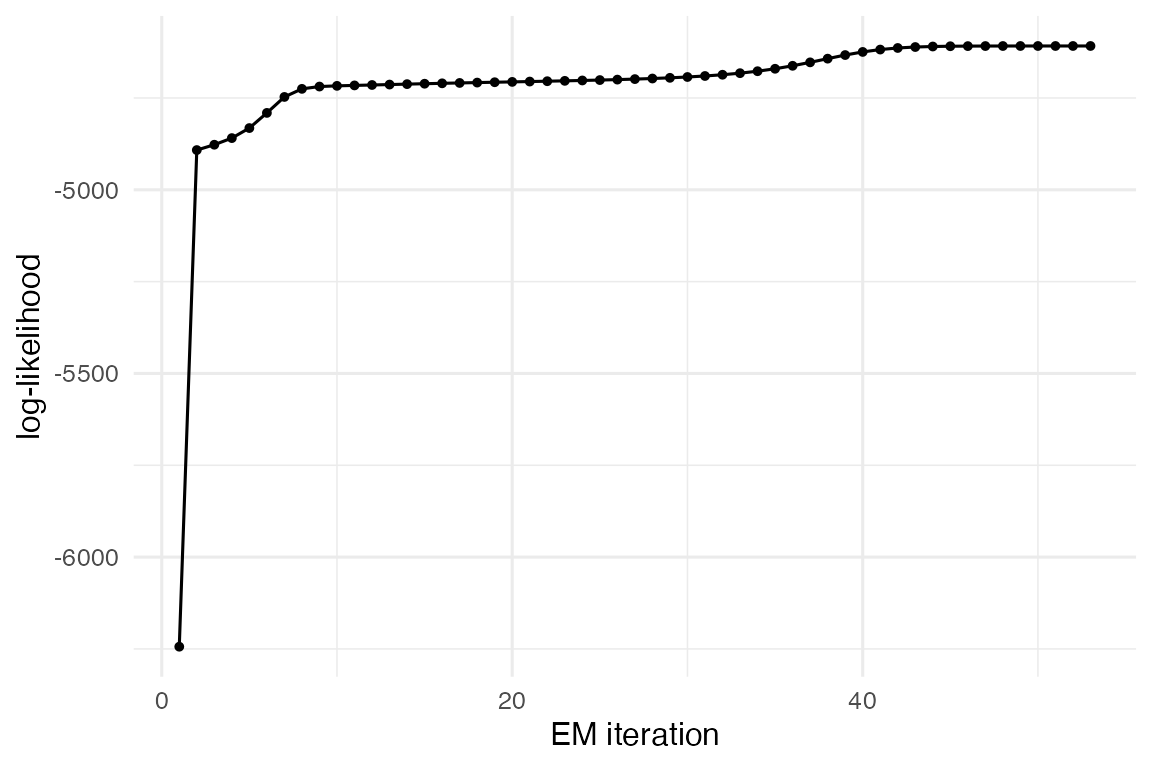
Sample-EM log-likelihood trace (monotone-up).
Information criteria are populated:
bic_aic(s_fit)
#> $bic
#> [1] 9341.256
#>
#> $aic
#> [1] 9250.931
#>
#> $icl
#> [1] 9644.749
#>
#> $classification_entropy
#> [1] 151.7466
#>
#> $n_params
#> [1] 17
Regime (iii): importance-sampled KLD-EM
Regime (iii) is the reason proxymix exists: it fits a
Gaussian-mixture proxy when the target’s log_density is
evaluable but no samples are available. Examples
include posterior distributions in Bayesian models, intractable
likelihoods, expensive simulators, and downscaling targets in spatial
statistics.
The algorithm:
- Draw
is_sizesamples from a user-supplied importance proposalq. - Compute self-normalised importance weights .
- Run EM iterations using the IS weights – the M-step minimises
by re-weighting responsibilities with
W.
The proposal q is the only free knob beyond the usual
mixture configuration; is_mvt() with df = 5 is
a robust default.
k_fit <- fit_proxymix(tgt, N = 3L, regime = "kld",
                      proposal = is_mvt(n_dim = 2L,
                                        mean = c(0, 0),
                                        sigma = 6 * diag(2),
                                        df = 5),
                      is_size = 3000L,
                      max_iter = 60L,
                      seed = 1L)
k_fit
#> <gmm_fit>: regime = "kld", K = 3, p = 2
#>   target     : three_mixture
#>   iterations : 10
#>   converged  : TRUE
#>   [1] w = 0.4164, |mu| = 0.0300, tr(Sigma) = 0.8377
#>   [2] w = 0.3069, |mu| = 2.7545, tr(Sigma) = 1.2249
#>   [3] w = 0.2767, |mu| = 2.7562, tr(Sigma) = 0.8740
Diagnostics:
trace <- kld_trace(k_fit)
if (requireNamespace("ggplot2", quietly = TRUE)) {
  ggplot(data.frame(iter = seq_along(trace), kld = trace),
         aes(iter, kld)) +
    geom_line() + geom_point(size = 1) +
    labs(x = "KLD-EM iteration", y = expression(widehat(KL)(f * "||" * g))) +
    theme_minimal(base_size = 12)
}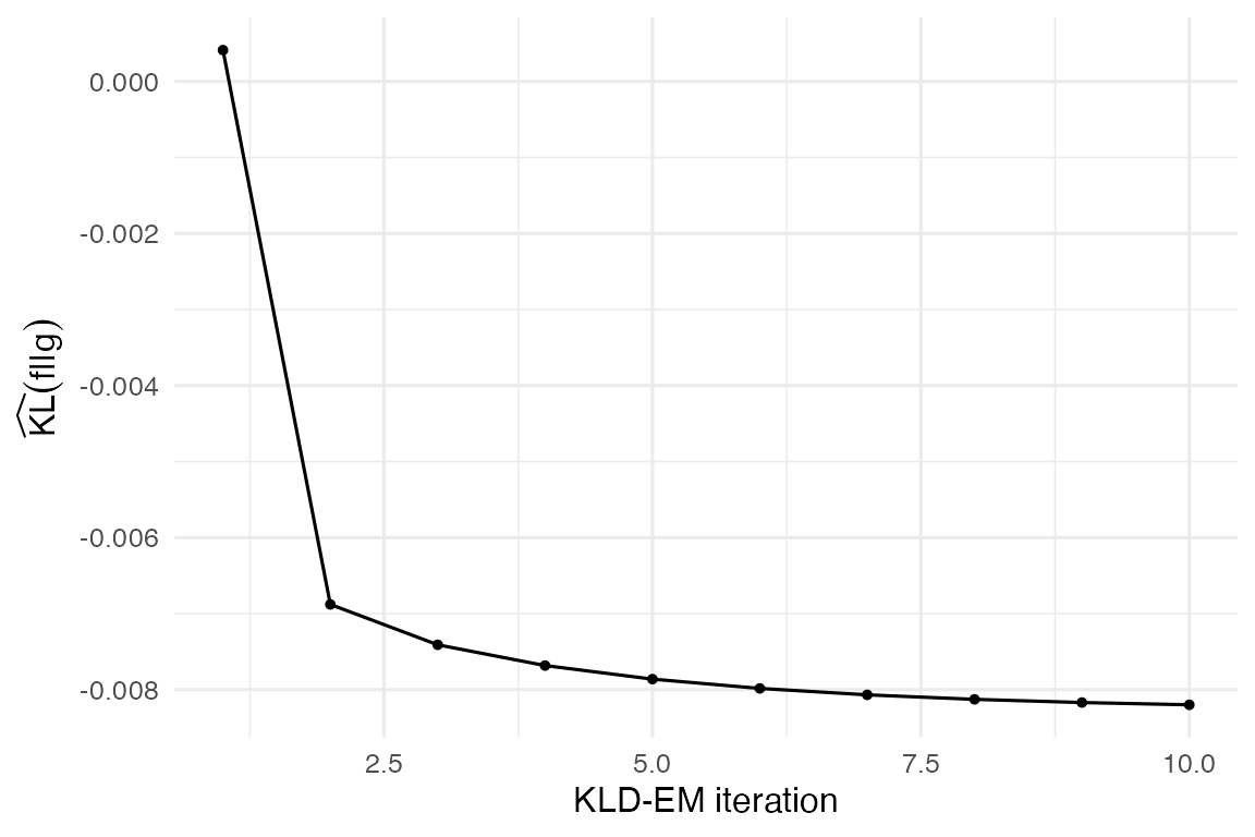
KLD-EM convergence trace.
Effective sample size of the importance weights:
ess_trace(k_fit)
#> [1] 757.7185
Side-by-side overlay
The three fits – moment (N = 1), classical EM (N = 3), KLD-EM (N = 3) – overlaid on the target:
if (requireNamespace("ggplot2", quietly = TRUE) &&
    requireNamespace("patchwork", quietly = TRUE)) {
  grid_x <- seq(-4.5, 4.5, length.out = 100)
  G <- expand.grid(x1 = grid_x, x2 = grid_x)
  G$f  <- exp(tgt@log_density(as.matrix(G)))
  G$mm <- exp(dgmm(as.matrix(G[, c("x1", "x2")]), m_fit, log = TRUE))
  G$ss <- exp(dgmm(as.matrix(G[, c("x1", "x2")]), s_fit, log = TRUE))
  G$kk <- exp(dgmm(as.matrix(G[, c("x1", "x2")]), k_fit, log = TRUE))

  base <- ggplot(G, aes(x1, x2)) +
    geom_contour_filled(aes(z = f), bins = 10L, alpha = 0.85) +
    scale_fill_viridis_d(option = "mako", guide = "none") +
    coord_equal() + theme_minimal(base_size = 11)

  p1 <- base + geom_contour(aes(z = mm), bins = 5L, colour = "white",
                            linetype = "dashed") +
    labs(title = "Regime (i) moment, N = 1", x = NULL, y = NULL)
  p2 <- base + geom_contour(aes(z = ss), bins = 5L, colour = "white",
                            linetype = "dashed") +
    labs(title = "Regime (ii) sample EM, N = 3", x = NULL, y = NULL)
  p3 <- base + geom_contour(aes(z = kk), bins = 5L, colour = "white",
                            linetype = "dashed") +
    labs(title = "Regime (iii) KLD-EM, N = 3", x = NULL, y = NULL)

  patchwork::wrap_plots(p1, p2, p3, nrow = 1)
}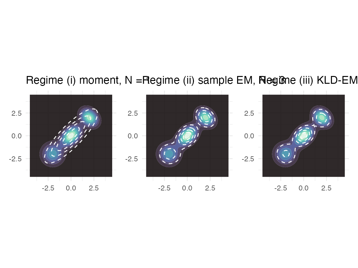
Target (filled) overlaid with the three regimes’ fits (dashed).
A sanity check: (i) and (iii) agree at N = 1
When N = 1, the KL-optimal Gaussian is the
moment-matched one. Regime (iii) – a numerical optimiser – should
converge to that same Gaussian (up to Monte Carlo error). Let us check
this on the banana target where regime (iii) is the only
available regime if we ignore samples:
banana <- banana_target(with_samples = TRUE, n = 2000L, seed = 1L)
m_b <- fit_proxymix(banana, N = 1L, regime = "moment")
k_b <- fit_proxymix(banana, N = 1L, regime = "kld",
                    proposal = is_mvt(n_dim = 2L,
                                      sigma = 4 * diag(2),
                                      df = 5),
                    is_size = 3000L, max_iter = 50L, seed = 1L)
rbind(
  moment_mean = m_b@means[[1L]],
  kld_mean    = k_b@means[[1L]]
)
#>                    [,1]       [,2]
#> moment_mean -0.01395503 0.05373059
#> kld_mean     0.01182980 0.01616172
rbind(
  moment_tr   = sum(diag(m_b@covariances[[1L]])),
  kld_tr      = sum(diag(k_b@covariances[[1L]]))
)
#>               [,1]
#> moment_tr 2.677815
#> kld_tr    2.447868
The means and trace-covariances agree to within Monte Carlo error.
Reference
Hoek, J. van der and Elliott, R. J. (2024). Mixtures of multivariate Gaussians. Stochastic Analysis and Applications. https://doi.org/10.1080/07362994.2024.2372605.