Mapping the optima of an objective

library(proxymix)

An objective is a density you can evaluate but not sample

An objective $f(x)$ to be minimised over a box defines an unnormalised density, the Gibbs measure $\exp(-f(x) / T)$, whose mass concentrates on the low regions of $f$ as the temperature $T$ falls. That density can be evaluated point-wise but not directly sampled, which is exactly regime (iii) of Hoek and Elliott (2024). from_objective() fits a Gaussian-mixture proxy to $\exp(-f / T)$ by cooling a short temperature ladder through the same importance-sampled KLD-EM that fit_kld_em() runs, warm-starting each step from the previous fit.

The point of the construction is not a single best point but the whole picture. A multimodal $f$ gives a multimodal Gibbs measure, so the fitted mixture spreads its components across the basins and recovers the optima together. The result is an ordinary gmm, so the closed-form operator calculus – marginalisation, conditioning, divergence – applies to the map of solutions. gmm_modes() reads the distinct optima off that map.

A bimodal objective in one dimension

The objective $(\theta^2 - 4)^2$ has two minima, at $\theta = -2$ and $\theta = 2$. We fit the map and resolve it.

f <- function(v) (v[1]^2 - 4)^2

fit <- from_objective(f, lower = -5, upper = 5, N = 6L,
                      is_size = 3000L, n_steps = 5L, seed = 1L)

modes <- gmm_modes(fit)
sort(round(modes$modes[, 1], 3))
#> [1] -2.006  2.019

Both minima are recovered. The fitted object is a gmm_fit, so the importance-sampling diagnostics are available alongside the map.

ess_summary(fit)
#> $is_size
#> [1] 3000
#> 
#> $ess
#> [1] 1577.087
#> 
#> $ess_relative
#> [1] 0.5256957
#> 
#> $max_weight
#> [1] 0.0009347261
#> 
#> $support_fraction
#> [1] 1
#> 
#> $mc_se_kld
#> [1] 0.001075373
#> 
#> $validation_size
#> [1] 0
#> 
#> $validation_ess
#> [1] NA
#> 
#> $validation_ess_relative
#> [1] NA
#> 
#> $validation_max_weight
#> [1] NA
#> 
#> $validation_support_fraction
#> [1] NA
#> 
#> $validation_kld
#> [1] NA

Four minima at once: Himmelblau

Himmelblau’s function has four equal minima. A single-point optimiser would return one of them and miss the rest. from_objective() returns all four in one fit, provided the number of components N is comfortably larger than the number of optima so that a component can settle on each basin.

himmelblau <- function(v) {
  x <- v[1]
  y <- v[2]
  (x * x + y - 11)^2 + (x + y * y - 7)^2
}

fit2 <- from_objective(himmelblau, lower = c(-5, -5), upper = c(5, 5),
                       N = 10L, is_size = 4000L, n_steps = 6L, seed = 1L)

found <- gmm_modes(fit2)
round(found$modes[order(found$modes[, 1]), ], 3)
#>        [,1]   [,2]
#> [1,] -3.756 -3.231
#> [2,] -2.734  3.096
#> [3,]  2.975  1.922
#> [4,]  3.533 -1.706

The four recovered minima sit at $(3, 2)$, $(-2.81, 3.13)$, $(-3.78, -3.28)$ and $(3.58, -1.85)$ – the known optima. The figure below overlays the recovered modes (orange) and the analytic truth (red crosses) on the log-objective surface.

truth <- rbind(c(3, 2), c(-2.805118, 3.131312),
               c(-3.779310, -3.283186), c(3.584428, -1.848126))

xs <- seq(-5, 5, length.out = 140)
ys <- seq(-5, 5, length.out = 140)
zz <- outer(xs, ys, Vectorize(function(a, b) himmelblau(c(a, b))))

image(xs, ys, log1p(zz), col = hcl.colors(40, "YlGnBu", rev = TRUE),
      xlab = expression(x[1]), ylab = expression(x[2]),
      main = "Himmelblau: the map over the four minima")
contour(xs, ys, log1p(zz), add = TRUE, col = "grey60",
        nlevels = 8, drawlabels = FALSE)
points(truth[, 1], truth[, 2], pch = 4, col = "red", cex = 2, lwd = 3)
points(found$modes[, 1], found$modes[, 2], pch = 19,
       col = "#D95F0E", cex = 1.4)
legend("topright", bg = "white",
       legend = c("analytic optima", "recovered modes"),
       pch = c(4, 19), col = c("red", "#D95F0E"),
       pt.cex = c(1.4, 1.2), pt.lwd = c(3, 1))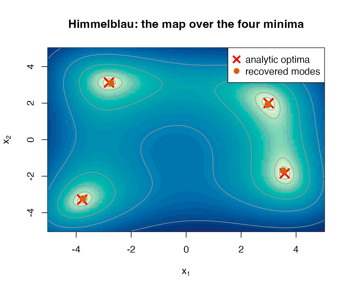

Notes on use

• Component headroom. Recovery is most reliable when N is larger than the number of optima. Symmetric landscapes, where several optima are exchangeable, need the most headroom. When in doubt raise N.
• The box is the search region. lower and upper set where the optima are sought and scale the temperature ladder, the uniform exploration of the proposal, and the initialisation. The objective may be evaluated outside the box during fitting, where non-finite values are treated as a finite penalty.
• Maximisation. Set minimise = FALSE to concentrate the map on the maxima of f instead of the minima.
• The map is a mixture. Because the return value is a gmm, the rest of the package applies. The optima can be conditioned, marginalised, or compared with gmm_divergence() like any other fitted mixture.

References

Hoek, J. van der and Elliott, R. J. (2024). Mixtures of multivariate Gaussians. Stochastic Analysis and Applications. doi:10.1080/07362994.2024.2372605.

Carreira-Perpinan, M. A. (2000). Mode-finding for mixtures of Gaussian distributions. IEEE Transactions on Pattern Analysis and Machine Intelligence, 22(11), 1318-1323.