Affine-Gaussian operator calculus on a Gaussian mixture

library(proxymix)
library(ggplot2)

Why an operator calculus

A fitted Gaussian-mixture proxy supports four kinds of downstream operations in closed form:

Pushforward through a linear sensor or aggregation operator (gmm_affine, gmm_aggregate).
Bayesian update on a noisy linear observation (gmm_observe – the finite-mixture analogue of a Kalman update).
Marginalisation over a coordinate subset (gmm_marginalise, shipped since v0.1).
Conditioning on fully observed coordinates (gmm_conditionalise, gmm_missing).

Each operator returns a gmm, so the operators compose freely without ever leaving closed form. This is the algebraic dividend of having fitted a parametric proxy in the first place – a non-parametric KDE or a Monte Carlo sample bank cannot do this.

A worked example

Start with a 2D mixture proxy of a pair of latent variables.

g_prior <- gmm(
  weights     = c(0.6, 0.4),
  means       = list(c(-1, 0), c(1.5, 0.5)),
  covariances = list(diag(c(0.6, 0.8)), diag(c(0.7, 0.5)))
)
g_prior
#> <gmm>: K = 2 components in p = 2 dimensions
#>   [1] w = 0.6000, |mu| = 1.0000, tr(Sigma) = 1.4000
#>   [2] w = 0.4000, |mu| = 1.5811, tr(Sigma) = 1.2000

Pushforward through a linear sensor

Suppose we observe $y = A x + \epsilon$ with $\epsilon \sim \mathcal{N}(0, R)$ and sensor matrix

A <- matrix(c(1, 0,
              0, 1,
              1, 1), nrow = 3L, byrow = TRUE)
b <- c(0, 0, 0)
R <- 0.05 * diag(3)

gmm_affine() returns the pushed-forward mixture in R^3.

g_pushed <- gmm_affine(g_prior, A, b, noise_cov = R)
g_pushed
#> <affine(gmm)>: K = 2 components in p = 3 dimensions
#>   [1] w = 0.6000, |mu| = 1.4142, tr(Sigma) = 2.9500
#>   [2] w = 0.4000, |mu| = 2.5495, tr(Sigma) = 2.5500

The weights are unchanged; the means are $A \mu_k + b$ and the covariances are $A \Sigma_k A^\top + R$ . The output is a closed-form mixture in the sensor space.

Bayesian update on a noisy linear observation

Suppose now that we observe y = 0.8 on the first coordinate of x alone, with noise variance R = 0.25.

A_obs <- matrix(c(1, 0), nrow = 1L)
g_post <- gmm_observe(g_prior, A = A_obs, y = 0.8,
                      noise_cov = matrix(0.25, 1L, 1L))
g_post
#> <observe(gmm)>: K = 2 components in p = 2 dimensions
#>   [1] w = 0.2338, |mu| = 0.2706, tr(Sigma) = 0.9765
#>   [2] w = 0.7662, |mu| = 1.1039, tr(Sigma) = 0.6842

Component weights have been multiplied by the marginal evidence $\pi_k \, \mathcal{N}(y;\, A \mu_k,\, S_k)$ and renormalised. Component means and covariances have been Kalman-updated component-wise.

Visualise the prior and the posterior on a planar grid:

grid <- expand.grid(x = seq(-4, 5, length.out = 80L),
                    y = seq(-3, 3, length.out = 60L))
gm <- as.matrix(grid)
prior_df <- data.frame(x = grid$x, y = grid$y,
                       d = dgmm(gm, g_prior), part = "prior")
post_df  <- data.frame(x = grid$x, y = grid$y,
                       d = dgmm(gm, g_post),  part = "posterior")
long <- rbind(prior_df, post_df)
long$part <- factor(long$part, levels = c("prior", "posterior"),
                    labels = c("Prior", "Posterior"))
ggplot(long, aes(x, y)) +
  geom_raster(aes(fill = d), interpolate = TRUE) +
  geom_contour(aes(z = d), colour = "white", linewidth = 0.2, alpha = 0.6,
               bins = 8L) +
  facet_wrap(~ part) +
  coord_equal(expand = FALSE) +
  scale_fill_viridis_c(name = "Density") +
  labs(title = expression(paste("Prior vs posterior after observing ",
                                y[1] == 0.8, "  (", sigma == 0.5, ")")),
       x = expression(x[1]), y = expression(x[2])) +
  theme_minimal(base_size = 11) +
  theme(plot.title = element_text(face = "bold", size = rel(1)),
        strip.text = element_text(face = "bold"),
        panel.grid = element_blank(),
        legend.position = "right")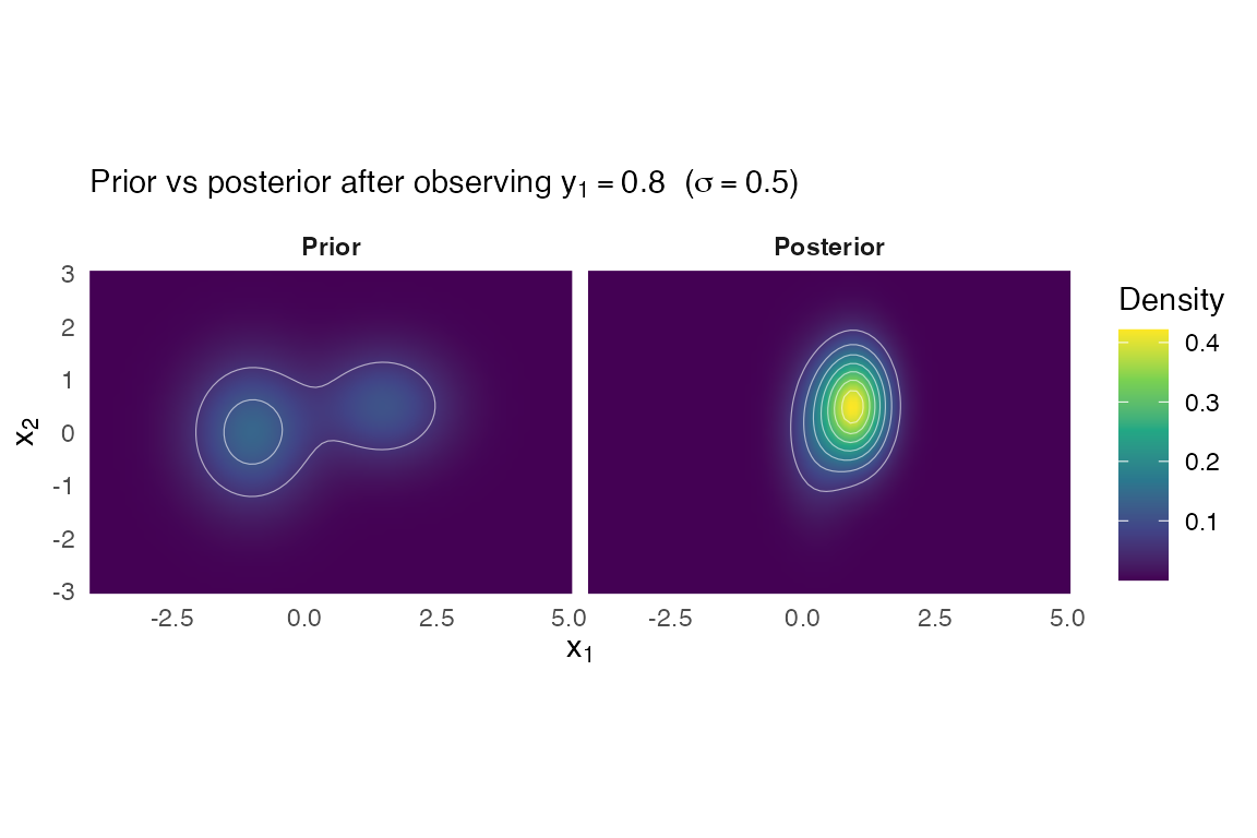

Kalman parity check

For a single-component prior, gmm_observe() collapses exactly to a Kalman update. Verify:

g_single <- gmm(
  weights     = 1,
  means       = list(c(0, 0)),
  covariances = list(diag(c(1, 2)))
)
g_one_obs <- gmm_observe(
  g_single,
  A = matrix(c(1, 0), nrow = 1L),
  y = 0.5,
  noise_cov = matrix(0.5, 1L, 1L)
)

## Hand Kalman:
S      <- diag(c(1, 2))
H      <- matrix(c(1, 0), nrow = 1L)
R_obs  <- matrix(0.5, 1L, 1L)
Sx     <- H %*% S %*% t(H) + R_obs
gain   <- S %*% t(H) %*% solve(Sx)
mu_hat <- as.numeric(gain * 0.5)
S_hat  <- S - gain %*% H %*% S

list(
  mu_diff_max  = max(abs(mu_hat - g_one_obs@means[[1L]])),
  cov_diff_max = max(abs(S_hat  - g_one_obs@covariances[[1L]]))
)
#> $mu_diff_max
#> [1] 1.110223e-16
#> 
#> $cov_diff_max
#> [1] 1e-06

The differences are at the level of the numerical-hygiene ridge (1e-6), so the operator is exact up to numerical tolerance.

Aggregation through a coarsening matrix

Aggregating a fine-grained latent (3 components) into a coarser one (sum of the first two coordinates) is a special case of gmm_affine with a row-sum A.

g_fine <- gmm(
  weights     = c(0.3, 0.4, 0.3),
  means       = list(c(0, 0, 0), c(2, 1, -1), c(-1, -1, 2)),
  covariances = list(diag(3), diag(3), diag(3))
)
A_agg <- matrix(c(1, 1, 0,
                  0, 0, 1), nrow = 2L, byrow = TRUE)
gmm_aggregate(g_fine, A_agg)
#> <aggregate(gmm)>: K = 3 components in p = 2 dimensions
#>   [1] w = 0.3000, |mu| = 0.0000, tr(Sigma) = 3.0000
#>   [2] w = 0.4000, |mu| = 3.1623, tr(Sigma) = 3.0000
#>   [3] w = 0.3000, |mu| = 2.8284, tr(Sigma) = 3.0000

The aggregated mixture has the same number of components and weights as the fine one, but with mu and Sigma mapped through A.

Missing-data conditioning

If a subset of coordinates is exactly observed (no noise), gmm_missing() routes through the Schur-complement path:

gmm_missing(g_prior, observed = 2L, values = 0.5)
#> <missing(gmm)>: K = 2 components in p = 1 dimensions
#>   [1] w = 0.5036, |mu| = 1.0000, tr(Sigma) = 0.6000
#>   [2] w = 0.4964, |mu| = 1.5000, tr(Sigma) = 0.7000

This is equivalent to gmm_conditionalise(g_prior, given = c(NA, 0.5)) but with a clearer index-based signature for missing-data pipelines.

Filtering over time – the Kalman filter as a special case

The Bayesian update above is a single step. A filter alternates two steps over time: a predict step that pushes the state forward through the dynamics (gmm_affine, the Chapman–Kolmogorov propagation of a linear stochastic dynamical system), and an update step that folds in each noisy measurement (gmm_observe). Run on a single-component prior, this recursion is the classical discrete-time Kalman filter; run on a multi-component prior, it is the Gaussian-sum filter – a bank of Kalman filters carried in parallel.

Take a one-dimensional constant-velocity track, with state $(\text{position}, \text{velocity})$ , linear dynamics $A$ , process noise $Q$ , and a noisy position sensor $C = [1, 0]$ with noise $R$ .

dt <- 1
A  <- matrix(c(1, dt, 0, 1), 2L, 2L, byrow = TRUE)   # constant velocity
C  <- matrix(c(1, 0), 1L, 2L)                         # observe position only
Q  <- 0.01 * diag(2)                                  # process noise
R  <- matrix(0.5, 1L, 1L)                             # sensor noise
set.seed(42)
n <- 30L
truth <- matrix(0, n, 2L)
truth[1L, ] <- c(0, 1)
for (k in 2:n) {
  truth[k, ] <- as.numeric(A %*% truth[k - 1L, ]) + mvnfast::rmvn(1L, c(0, 0), Q)
}
y <- truth[, 1L] + rnorm(n, 0, sqrt(R[1L, 1L]))       # noisy position readings

The filter is the operator calculus in a loop – gmm_affine() to predict, gmm_observe() to update:

g <- gmm(weights = 1, means = list(c(0, 0)), covariances = list(diag(2)))
filtered <- numeric(n)
for (k in seq_len(n)) {
  if (k > 1L) g <- gmm_affine(g, A = A, b = c(0, 0), noise_cov = Q)  # predict
  g <- gmm_observe(g, A = C, y = y[k], noise_cov = R)                # update
  filtered[k] <- g@means[[1L]][1L]
}

Against a hand-coded textbook Kalman filter the two tracks agree to the level of the numerical-hygiene ridge:

mu <- c(0, 0); S <- diag(2); kf <- numeric(n)
for (k in seq_len(n)) {
  if (k > 1L) { mu <- as.numeric(A %*% mu); S <- A %*% S %*% t(A) + Q }  # predict
  K  <- S %*% t(C) %*% solve(C %*% S %*% t(C) + R)                       # gain
  mu <- mu + as.numeric(K %*% (y[k] - C %*% mu))
  S  <- (diag(2) - K %*% C) %*% S
  kf[k] <- mu[1L]
}
c(max_abs_diff = max(abs(filtered - kf)))
#> max_abs_diff 
#> 4.803363e-05

track <- data.frame(t = seq_len(n), truth = truth[, 1L], y = y,
                    filtered = filtered)
ggplot(track, aes(t)) +
  geom_point(aes(y = y, colour = "noisy reading"), size = 1.3, alpha = 0.7) +
  geom_line(aes(y = truth, colour = "latent truth"), linewidth = 0.8) +
  geom_line(aes(y = filtered, colour = "filtered (K = 1)"), linewidth = 0.9) +
  scale_colour_manual(name = NULL,
                      values = c("noisy reading" = "grey55",
                                 "latent truth" = "#2C7FB8",
                                 "filtered (K = 1)" = "#D95F0E")) +
  labs(title = "Predict + update over time is a Kalman filter",
       x = "time step", y = "position") +
  theme_minimal(base_size = 11) +
  theme(legend.position = "top", plot.title = element_text(face = "bold"))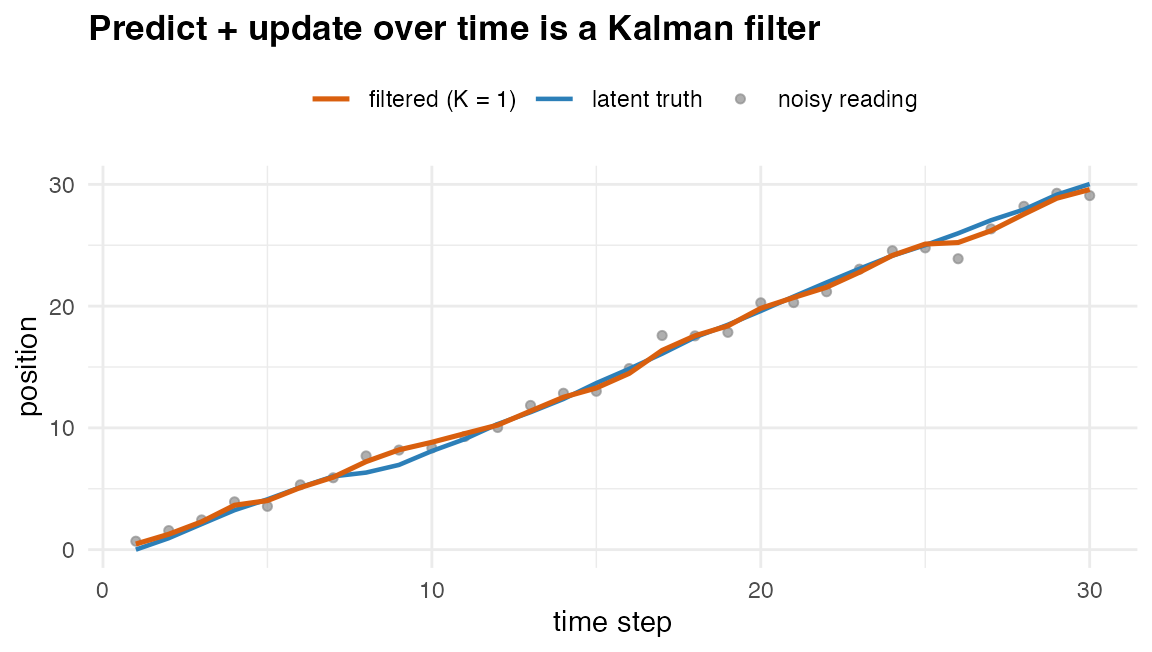

Time series with scattered noisy position readings, the smooth latent truth line, and the filtered estimate line tracking the truth.

A constant-velocity track filtered by the K = 1 operator-calculus recursion (the Kalman filter): noisy readings, the latent truth, and the filtered estimate.

The mixture generalisation. At $K > 1$ the same two calls run a Kalman filter inside every component and reweight the components by their evidence – the Gaussian-sum filter. It represents beliefs a single Kalman filter cannot (multimodal posteriors: several competing hypotheses about where the target is), at the cost that each gmm_observe (under a Gaussian-mixture noise or dynamics model) can multiply the component count. Collapsing the mixture back to a fixed budget keeps the filter bounded; that collapse is gmm_reduce(), next.

Bounding the filter – mixture reduction

gmm_reduce() collapses a mixture to a budget of at most k_max components by a greedy, moment-preserving pairwise merge: at each step the cheapest pair is replaced by the single Gaussian that preserves their combined weight, mean and covariance. Two merge costs decide which pair goes first – the Kullback–Leibler bound of Runnalls (2007), cost = "kl", and a closed-form Cauchy–Schwarz cost, cost = "cs", built from the same Gaussian-product identity as gmm_divergence().

Take a six-component mixture that really has three clusters, each split into two near-identical components, and reduce it to three:

g6 <- gmm(
  weights     = rep(1 / 6, 6),
  means       = list(c(-5, 0), c(-5, 0.15), c(5, 0), c(5.1, -0.1),
                     c(0, 6), c(0.1, 6.1)),
  covariances = rep(list(0.5 * diag(2)), 6)
)
g3 <- gmm_reduce(g6, k_max = 3L)
gmm_n_components(g3)
#> [1] 3

Because every merge is moment-preserving, the reduction leaves the mixture’s global mean and covariance untouched – and merging near-duplicates barely moves the mixture, so the divergence from the original is negligible:

mix_mean <- function(g) Reduce(`+`, Map(`*`, g@weights, g@means))
c(mean_shift = max(abs(mix_mean(g6) - mix_mean(g3))),
  divergence = gmm_divergence(g6, g3, type = "cs"))
#>   mean_shift   divergence 
#> 0.000000e+00 2.464851e-10

Reducing all the way to a single component returns the moment-matched Gaussian, so gmm_reduce() interpolates between the full mixture and its single-Gaussian summary. For a smooth, over-parameterised mixture a globally fitted proxy can beat any sequence of pairwise merges; method = "anneal" refits a budget-sized proxy by annealed EM and keeps it when it improves on the merge. In a Gaussian-sum filter, reduction runs after each update, holding the component count at the budget.

A bounded filter in one call – `gmm_filter()`

The predict / update / reduce loop is packaged as a single verb. gmm_filter() takes the prior belief, the linear-Gaussian dynamics and measurement, the observation series y, and an optional component cap k_max. With Gaussian noise and k_max = NULL it is the Kalman filter; with a Gaussian-sum process or measurement noise – a gmm in place of a covariance matrix – it is the Gaussian-sum filter, bounded by gmm_reduce() after each step.

On the constant-velocity track above, the verb reproduces the explicit Kalman recursion to machine precision (using the same predict-then-update convention):

prior <- gmm(weights = 1, means = list(c(0, 0)), covariances = list(diag(2)))
out <- gmm_filter(prior,
                  dynamics    = list(A = A, Q = Q),
                  measurement = list(C = C, R = R),
                  y = y, ridge_eps = 0)

mu <- c(0, 0); P <- diag(2); kf2 <- numeric(n)
for (k in seq_len(n)) {
  mu <- as.numeric(A %*% mu); P <- A %*% P %*% t(A) + Q          # predict
  G  <- P %*% t(C) %*% solve(C %*% P %*% t(C) + R)               # gain
  mu <- mu + as.numeric(G %*% (y[k] - C %*% mu))                 # update
  P  <- (diag(2) - G %*% C) %*% P
  kf2[k] <- mu[1L]
}
c(max_abs_diff = max(abs(out$mean[, 1L] - kf2)))
#> max_abs_diff 
#> 3.552714e-15

A heavy-tailed disturbance is awkward for a single Gaussian process noise. Modelled as a two-component Gaussian sum – a calm regime and an occasional larger jump – the recursion becomes a genuine Gaussian-sum filter. Each step multiplies the component count by two, so the cap returns it to budget:

q_heavy <- gmm(weights     = c(0.9, 0.1),
               means       = list(c(0, 0), c(0, 0)),
               covariances = list(0.01 * diag(2), 0.5 * diag(2)))
gsf <- gmm_filter(prior,
                  dynamics    = list(A = A, Q = q_heavy),
                  measurement = list(C = C, R = R),
                  y = y, k_max = 6L)
c(max_components = max(gsf$summary$n_components), steps = nrow(gsf$summary))
#> max_components          steps 
#>              6             30

The component count is held at the cap across the whole series. The $summary data frame records the filtered mean, standard deviation and component count at each step, and $filtered holds the full filtered mixture per step for any downstream closed-form query.

gsf_track <- data.frame(t = seq_len(n), truth = truth[, 1L], y = y,
                        filtered = gsf$mean[, 1L])
ggplot(gsf_track, aes(t)) +
  geom_point(aes(y = y, colour = "noisy reading"), size = 1.3, alpha = 0.7) +
  geom_line(aes(y = truth, colour = "latent truth"), linewidth = 0.8) +
  geom_line(aes(y = filtered, colour = "Gaussian-sum filter"), linewidth = 0.9) +
  scale_colour_manual(name = NULL,
                      values = c("noisy reading" = "grey55",
                                 "latent truth" = "#2C7FB8",
                                 "Gaussian-sum filter" = "#D95F0E")) +
  labs(title = "A bounded Gaussian-sum filter via gmm_filter()",
       x = "time step", y = "position") +
  theme_minimal(base_size = 11) +
  theme(legend.position = "top", plot.title = element_text(face = "bold"))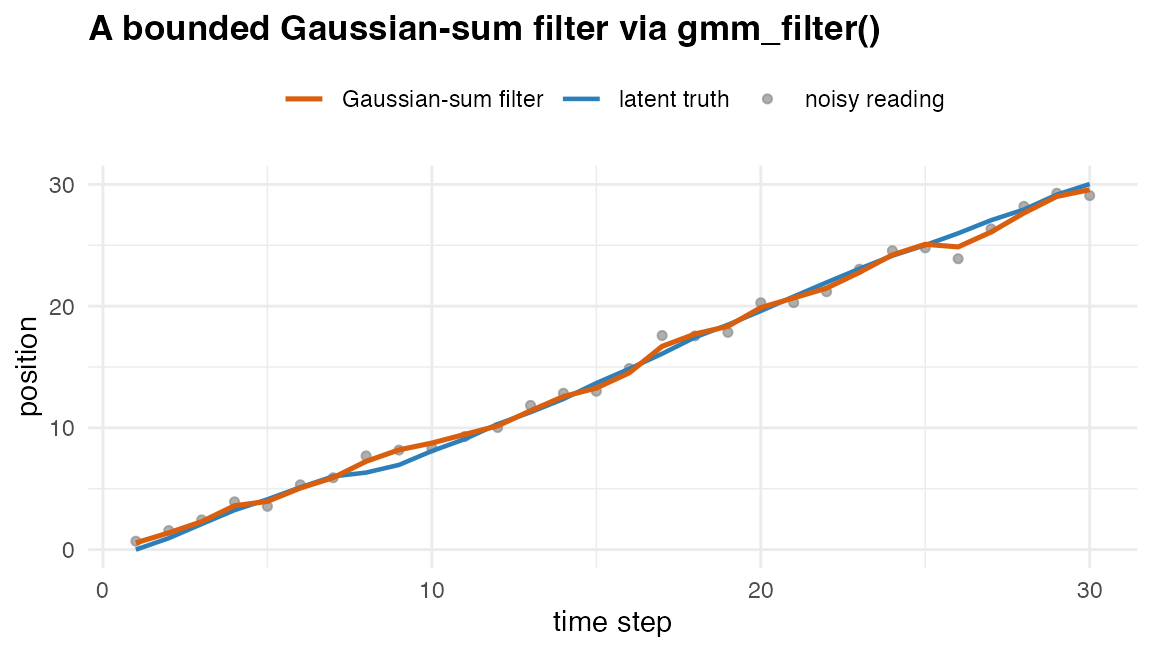

Time series with noisy position readings, the latent truth line, and the Gaussian-sum-filter estimate tracking the truth.

The same track filtered by the Gaussian-sum filter with a two-component heavy-tailed process noise, capped at six components per step. The filtered mean tracks the latent truth while the component count stays bounded.

Composition rules

The operators commute exactly with gmm_marginalise() when applied to disjoint coordinate subsets, and they associate under sequential observation:

## Two sequential observations on disjoint coordinates
g_a <- gmm_observe(g_prior, A = matrix(c(1, 0), nrow = 1L),
                   y = 0.5, noise_cov = matrix(0.25, 1, 1))
g_ab <- gmm_observe(g_a,    A = matrix(c(0, 1), nrow = 1L),
                    y = 0.2, noise_cov = matrix(0.25, 1, 1))

## Equivalent: one observation on the stacked coordinates
g_stack <- gmm_observe(
  g_prior,
  A         = diag(2),
  y         = c(0.5, 0.2),
  noise_cov = 0.25 * diag(2)
)

list(
  weights_diff = max(abs(g_ab@weights - g_stack@weights)),
  mu1_diff     = max(abs(g_ab@means[[1L]] - g_stack@means[[1L]])),
  cov1_diff    = max(abs(g_ab@covariances[[1L]] - g_stack@covariances[[1L]]))
)
#> $weights_diff
#> [1] 3.048779e-08
#> 
#> $mu1_diff
#> [1] 4.535143e-08
#> 
#> $cov1_diff
#> [1] 1e-06

The disagreement is at the ridge level – the two routes coincide.

When to not use the operator calculus

Non-linear channels. The closed-form maths uses linearity of A and Gaussianity of the noise. A non-linear sensor (e.g. a Sigmoid observation, a max-pooling aggregator) is not closed form and must not be silently approximated; use a Monte Carlo pushforward instead.
Non-Gaussian observation noise. Same restriction.
Hierarchical / random-effect models. The operator calculus applies to a fixed affine-Gaussian channel; a mixture-of-channels prior on (A, R) requires additional integration that is not closed form in general.

Comparison to a Gaussian-process latent

For a downscaling problem $g(y) = \mathbb{E}_{x \mid y}[f(x)]$ :

A Gaussian-process latent for f(x) gives a fully non-parametric, uncertainty-rich representation, and integration through a linear operator with additive Gaussian noise is closed form for a GP too. What it lacks is the cheap composition: repeatedly conditioning, aggregating, and re-mixing GP posteriors across configurations carries a growing kernel-algebra burden, where the mixture calculus stays a finite parameter list.
A finite Gaussian-mixture latent (what proxymix ships) is less flexible but admits the full operator calculus on this page. The trade-off is bias against algebraic tractability. The choice depends on how much closed-form composition the downstream pipeline needs.

References

Hoek, J. van der and Elliott, R. J. (2024). Mixtures of multivariate Gaussians. Stochastic Analysis and Applications. doi:10.1080/07362994.2024.2372605.
Kalman, R. E. (1960). A new approach to linear filtering and prediction problems. Transactions of the ASME – J. Basic Engineering.
Alspach, D. L. and Sorenson, H. W. (1972). Nonlinear Bayesian estimation using Gaussian sum approximations. IEEE Transactions on Automatic Control 17(4), 439–448.
Runnalls, A. R. (2007). Kullback–Leibler approach to Gaussian mixture reduction. IEEE Transactions on Aerospace and Electronic Systems 43(3), 989–999.
Murphy, K. P. (2012). Machine Learning: A Probabilistic Perspective. MIT Press. Ch. 4 (Gaussian models), Ch. 18 (state-space).