One mixture, many methods

library(proxymix)

A fitted Gaussian mixture over your data is a single object, and several classical analyses follow from it in closed form – because conditioning, marginalisation, and eigendecomposition are all exact on a Gaussian mixture. This vignette shows proxymix standing in for five familiar tools. Each section keeps the same shape: the problem, the usual tool, the proxymix route, the idea behind the substitution, and what it does and does not replace. The point is one fitted object serving several jobs, with the trade-offs in plain view – not that the mixture always wins.

Regression – from `lm()` to a conditioned mixture

Problem. Predict an outcome $y$ from a predictor $x$ . Usual tool. lm() / glm() – one global line. proxymix route. Fit a mixture over the joint $(y, x)$ , then read $E[y \mid x]$ by conditioning. At $K = 1$ this is least squares; at $K > 1$ the gate bends the line.

n <- 400L
x <- runif(n, -3, 3)
y <- 0.3 * x + 1.2 * pmax(x, 0) + rnorm(n, sd = 0.4)   # a bent relationship
dat <- data.frame(y = y, x = x)

joint <- gmm_target_from_samples(cbind(y, x))
fit1  <- fit_proxymix(joint, N = 1L, regime = "moment", ridge_eps = 0)   # = OLS
fit3  <- fit_proxymix(joint, N = 3L, regime = "sample", max_iter = 150L)

## At K = 1 the conditional slope equals the lm coefficient, exactly.
slope_mix <- gmm_conditionalise(fit1, given = c(NA, 1))@means[[1L]] -
  gmm_conditionalise(fit1, given = c(NA, 0))@means[[1L]]
c(proxymix = slope_mix, lm = unname(coef(lm(y ~ x, dat))["x"]))
#>  proxymix        lm 
#> 0.8968121 0.8968121

.cond_mean <- function(fit, xv) {
  vapply(xv, function(xx) {
    g <- gmm_conditionalise(fit, given = c(NA, xx))
    sum(g@weights * vapply(g@means, function(m) m[1L], numeric(1L)))
  }, numeric(1L))
}
if (requireNamespace("ggplot2", quietly = TRUE)) {
  library(ggplot2)
  grid <- data.frame(x = seq(-3, 3, length.out = 200L))
  grid$ols <- as.numeric(predict(lm(y ~ x, dat), newdata = grid))
  grid$mix <- .cond_mean(fit3, grid$x)
  ggplot() +
    geom_point(data = dat, aes(x, y), colour = "grey60", alpha = 0.4, size = 0.7) +
    geom_line(data = grid, aes(x, ols, colour = "lm (K = 1)"), linewidth = 0.9) +
    geom_line(data = grid, aes(x, mix, colour = "mixture (K = 3)"), linewidth = 0.9) +
    scale_colour_manual(name = NULL,
                        values = c("lm (K = 1)" = "#2C7FB8",
                                   "mixture (K = 3)" = "#D95F0E")) +
    labs(title = "Regression: one global line vs a conditioned mixture",
         x = expression(x), y = expression(y)) +
    theme_minimal(base_size = 11) +
    theme(legend.position = "top", plot.title = element_text(face = "bold"))
}

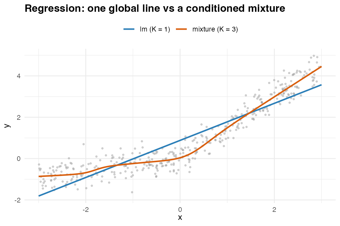
Scatter of y against x with the OLS line and the curved mixture conditional mean.

One global line (K = 1, = OLS) versus a conditioned mixture (K = 3).

Idea. Each component supplies an affine conditional mean $\mu_k^{y \mid x}$ ; the responsibilities $\pi_k(x)$ gate them, so the global mean $\sum_k \pi_k(x)\, \mu_k^{y \mid x}$ is nonlinear – Gaussian-mixture regression.

Does / does not. Captures nonlinear, heteroscedastic, even multimodal conditional densities, not just the mean. It does not return classical inference (standard errors, $p$ -values) by default, and it assumes Gaussian components.

Kernel regression – from Nadaraya–Watson to a conditioned KDE

Problem. Predict $y$ from $x$ with no global functional form – a purely local smoother. Usual tool. Nadaraya–Watson kernel regression (stats::ksmooth, package np): a kernel-weighted local average of the responses. proxymix route. Place one Gaussian per data point over the joint $(y, x)$ – a kernel density estimate – and read $E[y \mid x]$ by conditioning. With a Gaussian kernel that conditional mean is the Nadaraya–Watson estimator, exactly. Where lm() sat at $K = 1$ (one global line), Nadaraya–Watson sits at $K = n$ (one component per datum, fully local), and from_kde() lands anywhere in between – a single axis with least squares at one end and kernel smoothing at the other.

h <- 0.4                                       # kernel bandwidth
nw <- function(xq) vapply(xq, function(q) {
  w <- dnorm(q, x, h); sum(w * y) / sum(w)     # Nadaraya--Watson, Gaussian kernel
}, numeric(1L))

## One Gaussian per datum -- a kernel density estimate of the joint (y, x) --
## then condition on x and read the conditional mean.
kde <- gmm(weights = rep(1 / n, n),
           means = lapply(seq_len(n), function(i) c(y[i], x[i])),
           covariances = rep(list(diag(c(h^2, h^2))), n))
xq <- c(-2, -0.5, 1, 2.2)
c(max_abs_diff = max(abs(nw(xq) - .cond_mean(kde, xq))))   # equal to NW
#> max_abs_diff 
#> 3.552714e-15

if (requireNamespace("ggplot2", quietly = TRUE)) {
  grid_nw <- data.frame(x = seq(-3, 3, length.out = 200L))
  grid_nw$ols <- as.numeric(predict(lm(y ~ x, dat), newdata = grid_nw))
  grid_nw$nw  <- nw(grid_nw$x)
  ggplot() +
    geom_point(data = dat, aes(x, y), colour = "grey60", alpha = 0.4, size = 0.7) +
    geom_line(data = grid_nw, aes(x, ols, colour = "OLS (K = 1)"), linewidth = 0.9) +
    geom_line(data = grid_nw, aes(x, nw, colour = "kernel (K = n)"), linewidth = 0.9) +
    scale_colour_manual(name = NULL,
                        values = c("OLS (K = 1)" = "#2C7FB8",
                                   "kernel (K = n)" = "#D95F0E")) +
    labs(title = "From global line to local kernel, one conditioning operation",
         x = expression(x), y = expression(y)) +
    theme_minimal(base_size = 11) +
    theme(legend.position = "top", plot.title = element_text(face = "bold"))
}

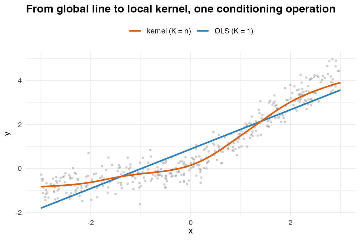
Scatter of y against x with the straight OLS line and the curved Nadaraya-Watson kernel-regression line.

One axis, two endpoints: the global line (K = 1, OLS) and the fully local kernel smoother (K = n, Nadaraya-Watson).

Idea. Conditioning a per-point KDE gives responsibilities $\pi_i(x) \propto \mathcal{N}(x \mid x_i, h^2)$ and per-component means $y_i$ , so $E[y \mid x] = \sum_i \pi_i(x)\, y_i$ – the Nadaraya–Watson ratio. Kernel regression is therefore Gaussian-mixture regression with one component per datum, a diagonal bandwidth, and only the conditional mean read off. The bandwidth $h$ plays the role of the component covariance.

Does / does not. The same operation returns the full conditional density (predictive variance, quantiles, multimodality), and gmm_conditional_entropy() scores its uncertainty – neither available from the bare Nadaraya–Watson mean. It also works in regime (iii), where you can evaluate the joint density but have no points to average, so a literal kernel estimator does not exist. The price is that the one-per-datum estimate costs $O(n)$ per query; from_kde() compresses it to a $K$ -component mixture for $O(K)$ queries, and – as with any kernel method – the bandwidth must be chosen.

Clustering – from `kmeans()` to the mixture components

Problem. Group rows by similarity. Usual tool. kmeans(), or mclust (which fits exactly this model). proxymix route. fit_proxymix(N = K, regime = "sample") – the components are the clusters and the responsibilities are soft assignments.

X <- rbind(
  mvnfast::rmvn(150L, c(-2, -1), 0.5 * diag(2)),
  mvnfast::rmvn(150L, c( 2,  0), matrix(c(0.6, 0.3, 0.3, 0.4), 2L)),
  mvnfast::rmvn(150L, c( 0,  2.5), 0.3 * diag(2))
)
colnames(X) <- c("V1", "V2")
ct   <- gmm_target_from_samples(X)
fitc <- fit_proxymix(ct, N = 3L, regime = "sample", max_iter = 150L)

## Soft assignment = posterior responsibility of each component.
.responsibilities <- function(fit, x) {
  comp <- vapply(seq_len(gmm_n_components(fit)), function(k) {
    fit@weights[k] *
      mvnfast::dmvn(x, mu = fit@means[[k]], sigma = fit@covariances[[k]])
  }, numeric(nrow(x)))
  comp / rowSums(comp)
}
resp <- .responsibilities(fitc, X)
head(round(resp, 3L), 3L)
#>       [,1] [,2]  [,3]
#> [1,] 0.000    0 1.000
#> [2,] 0.001    0 0.999
#> [3,] 0.001    0 0.999

Idea. Soft, model-based clustering: a point’s assignment to cluster $k$ is its posterior responsibility $\pi_k\,\mathcal{N}(x \mid \mu_k, \Sigma_k) / \sum_j \pi_j\,\mathcal{N}(x \mid \mu_j, \Sigma_j)$ .

Does / does not. Gives soft, full-covariance, density-aware clusters (ellipsoidal, not spherical like $k$ -means), and it doubles as a density estimate. It does not choose $K$ for you (use bic_aic()), and kmeans() is faster at very large $n$ .

Principal components – from `prcomp()` to the fitted covariance

Problem. Find the directions of greatest variation. Usual tool. prcomp(). proxymix route. Fit a single Gaussian (N = 1, regime = "moment") and eigendecompose its covariance.

fit_pca <- fit_proxymix(ct, N = 1L, regime = "moment", ridge_eps = 0)
ev <- eigen(fit_pca@covariances[[1L]])$vectors
pr <- prcomp(X)$rotation
## Identical to the prcomp rotation, up to the sign convention of each axis.
max(abs(abs(ev) - abs(unname(pr))))
#> [1] 5.551115e-16

if (requireNamespace("ggplot2", quietly = TRUE)) {
  vals <- eigen(fit_pca@covariances[[1L]])$values
  mu   <- fit_pca@means[[1L]]
  axes <- data.frame(
    x = mu[1L], y = mu[2L],
    xend = mu[1L] + 2 * sqrt(vals) * ev[1L, ],
    yend = mu[2L] + 2 * sqrt(vals) * ev[2L, ]
  )
  pts <- data.frame(X, cluster = factor(max.col(resp)))
  ggplot() +
    geom_point(data = pts, aes(V1, V2, colour = cluster), alpha = 0.6, size = 0.9) +
    geom_segment(data = axes, aes(x = x, y = y, xend = xend, yend = yend),
                 arrow = grid::arrow(length = grid::unit(0.2, "cm")),
                 linewidth = 0.8) +
    scale_colour_viridis_d(name = "cluster", end = 0.85) +
    coord_equal() +
    labs(title = "Clustering and principal axes from one mixture",
         x = expression(x[1]), y = expression(x[2])) +
    theme_minimal(base_size = 11) +
    theme(plot.title = element_text(face = "bold"))
}
#> Warning in data.frame(x = mu[1L], y = mu[2L], xend = mu[1L] + 2 * sqrt(vals) *
#> : row names were found from a short variable and have been discarded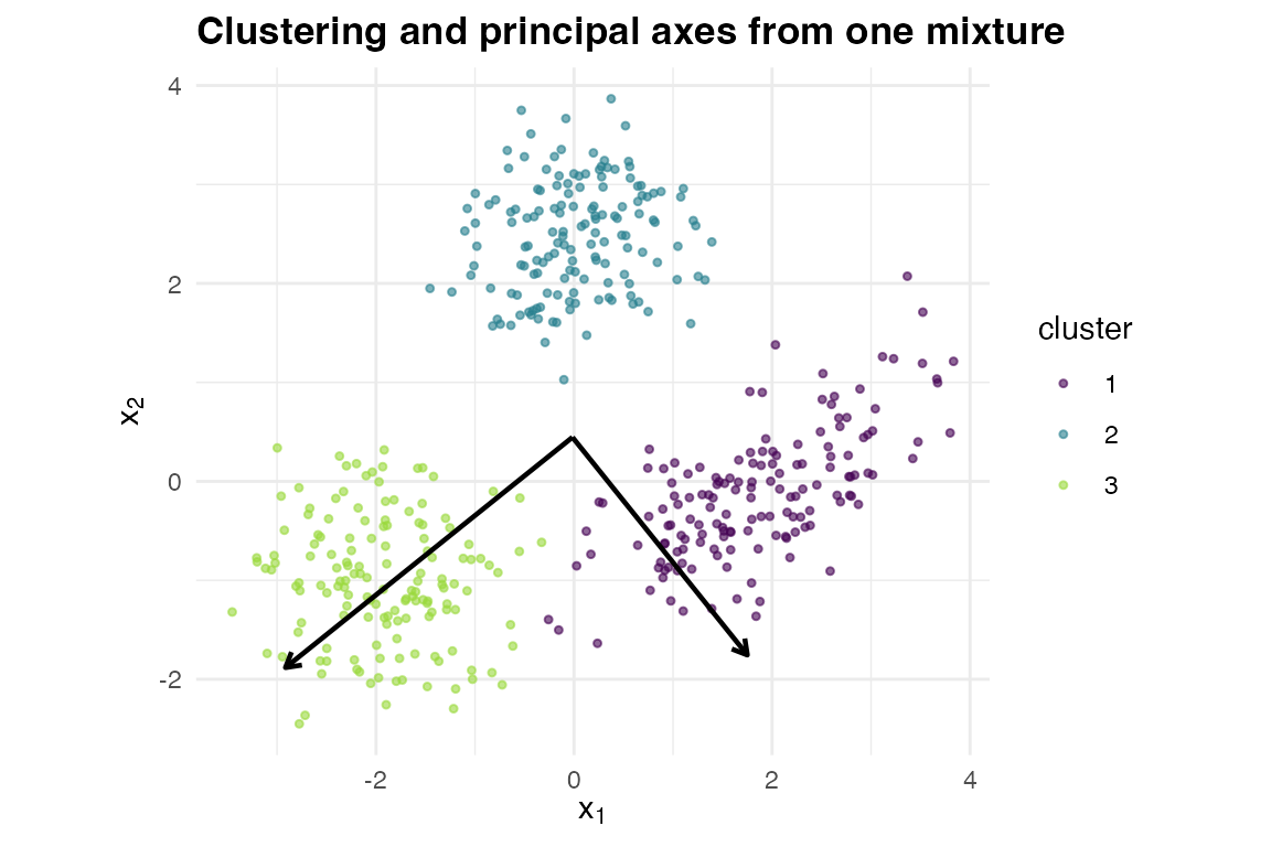

Three coloured point clusters with two principal-axis arrows from the centroid.

Clustering (colour) and the principal axes (arrows) read off one mixture.

Idea. PCA is the eigendecomposition of the covariance. The moment-matched single Gaussian carries the sample covariance exactly, so its eigenvectors are the principal components; with $K > 1$ you get a local PCA inside each cluster.

Does / does not. Recovers PCA exactly at $K = 1$ and a local PCA at $K > 1$ . For a one-off linear projection prcomp() is more direct – loadings, scree plots, and biplots come for free there.

Penalised regression – ridge as a covariance ridge

Problem. Stabilise a regression when predictors are collinear. Usual tool. glmnet (ridge / lasso), MASS::lm.ridge. proxymix route. The ridge_eps argument adds $\lambda I$ to the component covariance, which shrinks the conditional regression – exactly an $L_2$ (ridge) penalty.

lambda <- c(0, 0.5, 2, 8)
slope_pm <- vapply(lambda, function(lam) {
  f <- fit_proxymix(joint, N = 1L, regime = "moment", ridge_eps = lam)
  gmm_conditionalise(f, given = c(NA, 1))@means[[1L]] -
    gmm_conditionalise(f, given = c(NA, 0))@means[[1L]]
}, numeric(1L))
data.frame(
  lambda          = lambda,
  proxymix_slope  = round(slope_pm, 4L),
  ridge_formula   = round(cov(x, y) / (var(x) + lambda), 4L)
)
#>   lambda proxymix_slope ridge_formula
#> 1    0.0         0.8968        0.8968
#> 2    0.5         0.7680        0.7680
#> 3    2.0         0.5367        0.5367
#> 4    8.0         0.2434        0.2434

Idea. Conditioning gives $\beta = \Sigma_{xx}^{-1}\Sigma_{xy}$ . Ridging $\Sigma_{xx} \to \Sigma_{xx} + \lambda I$ yields $(\Sigma_{xx} + \lambda I)^{-1}\Sigma_{xy}$ – the ridge estimator – so the slope shrinks toward zero as $\lambda$ grows.

Does / does not. Delivers ridge-style shrinkage and numerical stability. There is no Gaussian-mixture analogue of the lasso: $L_2$ shrinkage matches a Gaussian prior, $L_1$ sparsity a Laplace prior that lies outside the Gaussian family – so proxymix does not perform variable selection.

A few more, in one line each

Imputation – gmm_conditionalise() on the observed coordinates gives the conditional-mean (or, via rgmm(), a sampled) fill-in.
Density estimation – the native use; from_kde() compresses a kernel estimate into a closed-form mixture (see vignette("from_kde")).
Kalman filtering – gmm_observe() is the mixture Kalman update (see vignette("operator_calculus")).

Summary

Method	Usual tool	`proxymix` route	What you gain	What you give up
Regression	`lm` / `glm`	mixture over $(y, x)$ + `gmm_conditionalise()`	nonlinear, heteroscedastic, multimodal conditional densities	built-in inference; Gaussian components
Kernel regression	`ksmooth` / `np` (Nadaraya–Watson)	per-point KDE + `gmm_conditionalise()`; compress with `from_kde()`	full conditional density, uncertainty, the evaluate-only regime	$O(n)$ per query unless compressed; bandwidth choice
Clustering	`kmeans` / `mclust`	`fit_proxymix(regime = "sample")`	soft, ellipsoidal, density-aware clusters	automatic $K$ ; speed at huge $n$
PCA	`prcomp`	`eigen()` of the `N = 1` covariance	local PCA per cluster at $K > 1$	loadings / scree / biplot conveniences
Ridge	`glmnet` / `lm.ridge`	`ridge_eps` on the covariance	$L_2$ shrinkage from one object	$L_1$ sparsity / variable selection

When to reach for the specialised tool

Use the purpose-built tool when its strengths are exactly what you need: high-dimensional sparse problems suit glmnet; very large- $n$ clustering suits kmeans; a single linear projection suits prcomp; classical inferential guarantees suit lm / glm. proxymix earns its place when you want one fitted object to serve several of these at once, in closed form, and when the Gaussian-mixture assumptions fit your data.

References

de Veaux, R. D. (1989). Mixtures of linear regressions. Computational Statistics & Data Analysis 8(3), 227–245.
Fraley, C. and Raftery, A. E. (2002). Model-based clustering, discriminant analysis, and density estimation. Journal of the American Statistical Association 97(458), 611–631.
Jolliffe, I. T. (2002). Principal Component Analysis, 2nd ed. Springer.
Nadaraya, E. A. (1964). On estimating regression. Theory of Probability and Its Applications 9(1), 141–142.
Watson, G. S. (1964). Smooth regression analysis. Sankhya A 26(4), 359–372.
Tipping, M. E. and Bishop, C. M. (1999). Probabilistic principal component analysis. Journal of the Royal Statistical Society B 61(3), 611–622.
Hoerl, A. E. and Kennard, R. W. (1970). Ridge regression: biased estimation for nonorthogonal problems. Technometrics 12(1), 55–67.
Hoek, J. van der and Elliott, R. J. (2024). Mixtures of multivariate Gaussians. Stochastic Analysis and Applications. doi:10.1080/07362994.2024.2372605.

Regression – from lm() to a conditioned mixture