proxymix fits Gaussian-mixture proxies to
user-supplied target densities. The unified verb is
fit_proxymix(target, N, regime = c("auto", "moment", "sample", "kld"))– and the three fitting regimes come from Hoek and Elliott (2024):
| Regime | When it applies | Method |
|---|---|---|
"moment" |
N == 1 and the target carries samples |
Closed-form moment matching |
"sample" |
N >= 2 and the target carries samples |
Classical EM |
"kld" |
The target carries log_density only |
Importance-sampled KLD-EM |
The "kld" regime is the reason the package exists: it
fits Gaussian-mixture proxies when you can evaluate f(x)
but cannot (cheaply) sample from it – the setting the sample-based
mixture packages (mclust, mixtools,
flexmix) do not address.
A target you cannot sample from
We use the bundled “banana” target – a non-Gaussian 2-D shape obtained by warping an isotropic Gaussian through a quadratic. Its log-density is exact and normalised; we deliberately do not attach samples, so only regime (iii) applies.
tgt <- banana_target()
tgt
#> <gmm_target>: "banana" in p = 2 dimensions
#>   log_density : supplied
#>   samples     : <absent>
#>   normalised  : TRUE
#>   log Z(f)    : 0
A quick look at the target as a contour grid:
grid_x <- seq(-3, 3, length.out = 120)
grid_y <- seq(-3, 3, length.out = 120)
G <- expand.grid(x1 = grid_x, x2 = grid_y)
G$f <- exp(tgt@log_density(as.matrix(G)))

if (requireNamespace("ggplot2", quietly = TRUE)) {
  library(ggplot2)
  ggplot(G, aes(x1, x2, z = f)) +
    geom_contour_filled(bins = 12L) +
    scale_fill_viridis_d(option = "mako", guide = "none") +
    coord_equal() +
    labs(title = "Banana target", x = expression(x[1]), y = expression(x[2])) +
    theme_minimal(base_size = 12)
}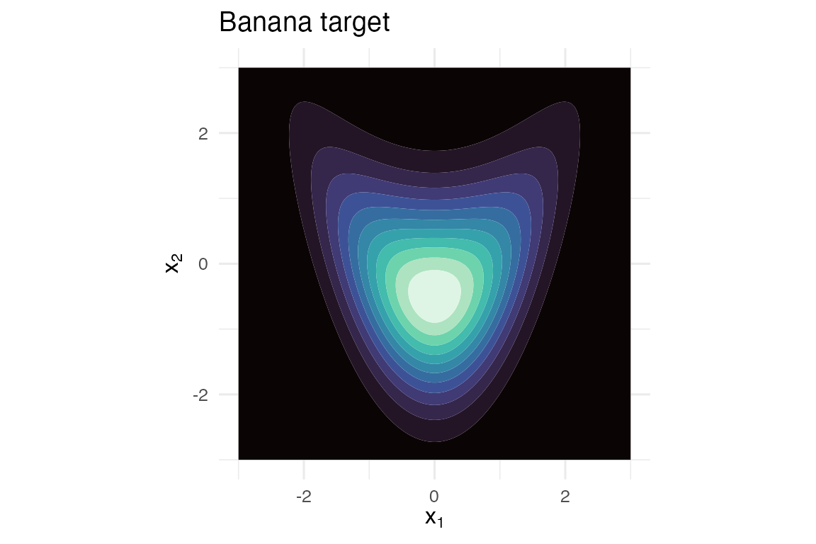
The banana target density.
Fit a Gaussian-mixture proxy
We fit a 3-component proxy by KLD-EM with importance sampling against a multivariate-Student-t proposal. The fit runs in a fraction of a second.
proposal <- is_mvt(n_dim = 2L, mean = c(0, 0),
                   sigma = 4 * diag(2), df = 5)

fit <- fit_proxymix(tgt, N = 3L, regime = "kld",
                    proposal = proposal,
                    is_size = 2000L,
                    max_iter = 30L,
                    seed = 1L)
fit
#> <gmm_fit>: regime = "kld", K = 3, p = 2
#>   target     : banana
#>   iterations : 30
#>   converged  : FALSE
#>   [1] w = 0.5239, |mu| = 0.2940, tr(Sigma) = 1.3436
#>   [2] w = 0.3190, |mu| = 0.9182, tr(Sigma) = 2.0353
#>   [3] w = 0.1571, |mu| = 1.4565, tr(Sigma) = 3.1361
Diagnostics:
data.frame(
  iter = seq_along(kld_trace(fit)),
  kld  = kld_trace(fit)
)
#>    iter         kld
#> 1     1 0.106304086
#> 2     2 0.054084708
#> 3     3 0.041219607
#> 4     4 0.034333212
#> 5     5 0.029677252
#> 6     6 0.026073076
#> 7     7 0.023038506
#> 8     8 0.020345599
#> 9     9 0.017883575
#> 10   10 0.015611379
#> 11   11 0.013535128
#> 12   12 0.011684420
#> 13   13 0.010085833
#> 14   14 0.008745624
#> 15   15 0.007647718
#> 16   16 0.006761492
#> 17   17 0.006051086
#> 18   18 0.005481955
#> 19   19 0.005024123
#> 20   20 0.004653134
#> 21   21 0.004349770
#> 22   22 0.004099261
#> 23   23 0.003890383
#> 24   24 0.003714640
#> 25   25 0.003565584
#> 26   26 0.003438288
#> 27   27 0.003328941
#> 28   28 0.003234560
#> 29   29 0.003152773
#> 30   30 0.003081664
ess_trace(fit)
#> [1] 820.6438
Overlay the proxy on the target
G$g <- exp(dgmm(as.matrix(G[, c("x1", "x2")]), fit, log = TRUE))

if (requireNamespace("ggplot2", quietly = TRUE)) {
  ggplot(G, aes(x1, x2)) +
    geom_contour_filled(aes(z = f), bins = 10L, alpha = 0.8) +
    geom_contour(aes(z = g), colour = "white", linetype = "dashed",
                 linewidth = 0.4, bins = 8L) +
    scale_fill_viridis_d(option = "mako", guide = "none") +
    coord_equal() +
    labs(title = "Target (filled) and proxy (dashed)",
         x = expression(x[1]), y = expression(x[2])) +
    theme_minimal(base_size = 12)
}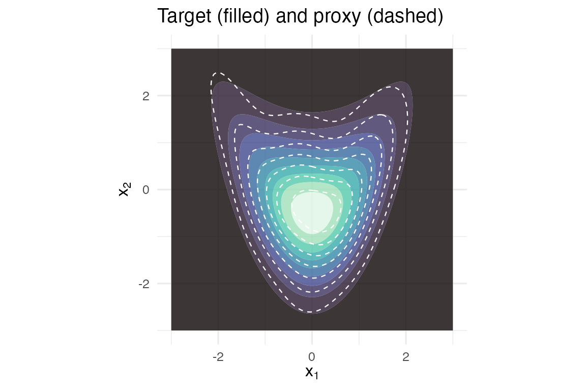
Banana target (filled) with the 3-component proxy overlaid (dashed contours).
Closed-form mixture operations
Because the fit is a Gaussian mixture, marginals and conditionals are closed-form and exact:
gmm_marginalise(fit, keep = 1L)
#> <marginalise(kld_em[N=3] on banana)>: K = 3 components in p = 1 dimensions
#>   [1] w = 0.5239, |mu| = 0.1790, tr(Sigma) = 0.4435
#>   [2] w = 0.3190, |mu| = 0.9167, tr(Sigma) = 0.4370
#>   [3] w = 0.1571, |mu| = 1.3103, tr(Sigma) = 0.5356
gmm_conditionalise(fit, given = c(NA, 0.5))
#> <conditionalise(kld_em[N=3] on banana)>: K = 3 components in p = 1 dimensions
#>   [1] w = 0.5508, |mu| = 0.2423, tr(Sigma) = 0.4368
#>   [2] w = 0.3186, |mu| = 1.0769, tr(Sigma) = 0.2332
#>   [3] w = 0.1305, |mu| = 1.2588, tr(Sigma) = 0.1612
You can sample from the proxy directly:
Where to next
-
vignette("three_regimes")– what each of regimes (i), (ii), (iii) does, with a head-to-head comparison on a target whose ground truth is known. -
vignette("density_shapes")– the regime-(iii) demonstration. KLD-EM fit on three different non-Gaussian targets (banana, donut, three-mixture), with KLD / ESS / Hellinger reported. -
vignette("operator_calculus")– closed-form pushforward, Bayesian update, aggregation and conditioning on a fitted mixture. -
vignette("from_kde")– compressing a kernel density estimate into a Gaussian-mixture proxy.
Reference
Hoek, J. van der and Elliott, R. J. (2024). Mixtures of multivariate Gaussians. Stochastic Analysis and Applications. https://doi.org/10.1080/07362994.2024.2372605.