Imputing missing data with a mixture

library(proxymix)

has_ggplot2 <- requireNamespace("ggplot2", quietly = TRUE)
has_mice <- requireNamespace("mice", quietly = TRUE)

The problem

An analyst has two measurements per unit. The scatter falls into two clear clusters with almost nothing between them, and a good half of the second measurement never came back from the field. The question is not whether an imputer will run. It is: my data has two clusters and an empty gap between them, so if I let a standard imputer fill the holes, will it put values in the gap where I know there is no mass, and will that move the mean I am going to report?

This vignette answers both halves on a synthetic two-cluster toy where the values that went missing are retained, so every imputation can be scored against the truth it was hiding.

Package capabilities

Imputation here is conditioning. If the joint distribution of the data is a Gaussian mixture, the conditional distribution of a missing entry given the observed entries of its own row is itself a Gaussian mixture, available in closed form through the Schur-complement algebra of gmm_conditionalise(). Nothing is simulated to get it.

gmm_impute() fits that mixture to a matrix containing holes and draws m completed datasets from the per-row conditionals. Its N argument is the number of mixture components, chosen by the Bayesian information criterion when left at its default. A mixture can be multimodal and can give each component its own spread, which neither a single-Gaussian model nor a linear-Gaussian conditional such as normal regression imputation can.

gmm_complete() extracts one completed dataset. proxy_pool() combines an estimand across the completions, and proxy_fmi() reports the fraction of missing information. For a column mean the pooling is closed form – the limit of the between-imputation variance as the number of completions m grows without bound – so no Monte Carlo noise enters at the pooling step. For any other estimand, as_mids() packages the completions as a mice object so the joint mixture imputations flow into mice::pool() unchanged: proxymix supplies the imputation model, mice the pooling.

Addressing the problem

A two-cluster toy with the truth retained

Two groups, each a tight cloud, with a positive within-group association between x1 and x2. This is a synthetic toy: the complete data is generated first and kept, then part of x2 is deleted, so the held-out values are available to score against. The chance of an entry going missing depends on the observed x1 and not on the hidden x2 itself, which is the missing-at-random setting.

set.seed(20260620)
n <- 600L
lab <- sample(c(-1, 1), n, replace = TRUE)
x1 <- 2 * lab + rnorm(n, 0, 0.6)
x2 <- 2 * lab + 0.5 * (x1 - 2 * lab) + rnorm(n, 0, 0.6)
truth <- cbind(x1 = x1, x2 = x2)

x_holes <- truth
missing <- runif(n) < plogis(0.6 * x1)
x_holes[missing, "x2"] <- NA
frac_missing <- mean(missing)

The marginal distribution of x2 is bimodal, one cluster near $-2$ and one near $+2$ , with little mass between them. Writing the empty middle as the interval $|x_2| < 1$ , the values that were deleted put only a small share of their mass there.

in_gap <- function(v) mean(abs(v) < 1)
gap_truth <- in_gap(truth[missing, "x2"])

Impute with a mixture, and with a single Gaussian

imp <- gmm_impute(x_holes, N = 2L, m = 20L, seed = 1L)
imp
#> <gmm_imputation>: m = 20 completions, K = 2 components, p = 2
#>   mechanism  : missing at random
#>   missing    : x1 0%, x2 53%

A single completed dataset has no holes:

done <- gmm_complete(imp, 1L)
anyNA(done)
#> [1] FALSE

Forcing one component reproduces the multivariate-normal assumption.

imp1 <- gmm_impute(x_holes, N = 1L, m = 20L, seed = 1L)
done1 <- gmm_complete(imp1, 1L)

How much mass each imputer places in the empty middle between the two clusters, over the 320 deleted entries. The two imputation rows are read from the first of the 20 completions of each imputer.
Source	Share of values with $\lvert x_2 \rvert < 1$
held-out truth	0.069
mixture imputation (N = 2)	0.084
single-Gaussian imputation (N = 1)	0.184

The shape of the imputations

dens_df <- function(v, label) {
  d <- density(v)
  data.frame(x2 = d$x, density = d$y, source = label,
             stringsAsFactors = FALSE)
}
plot_df <- rbind(
  dens_df(truth[missing, "x2"], "held-out truth"),
  dens_df(done[missing, "x2"], "mixture (N = 2)"),
  dens_df(done1[missing, "x2"], "single Gaussian (N = 1)")
)
plot_df$source <- factor(
  plot_df$source,
  levels = c("held-out truth", "mixture (N = 2)",
             "single Gaussian (N = 1)")
)
ggplot2::ggplot(plot_df, ggplot2::aes(x2, density, colour = source)) +
  ggplot2::geom_line(linewidth = 0.9) +
  ggplot2::annotate("rect", xmin = -1, xmax = 1, ymin = -Inf, ymax = Inf,
                    fill = "grey60", alpha = 0.18) +
  ggplot2::scale_colour_manual(
    name = NULL,
    values = c("held-out truth" = "#000000",
               "mixture (N = 2)" = "#009E73",
               "single Gaussian (N = 1)" = "#D55E00")
  ) +
  ggplot2::labs(
    x = expression(x[2]), y = "density",
    title = "What each imputer put where the data was deleted",
    subtitle = expression("Shaded band marks the empty middle, " *
                            group("|", x[2], "|") < 1)
  ) +
  ggplot2::theme_minimal(base_size = 11) +
  ggplot2::theme(legend.position = "top")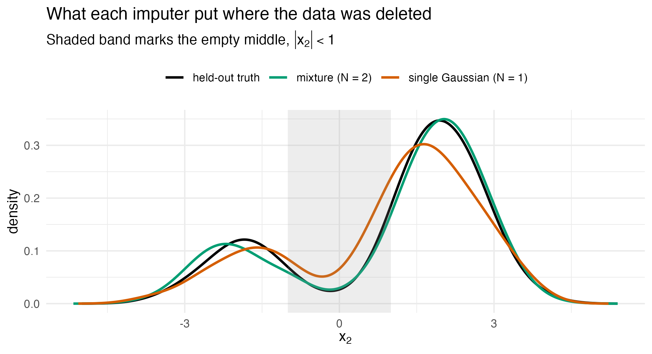

Three density curves over x2: the held-out truth, the mixture imputation and the single-Gaussian imputation are all bimodal; the single-Gaussian curve has lower peaks set closer to the middle and more density in the shaded gap between the two clusters.

Density of the deleted $x_2$ values against the values each imputer supplied in their place. The truth peaks at $x_2$ = $-1.84$ and $1.94$ , the mixture imputation at $-2.21$ and $2.03$ , and the single-Gaussian imputation at $-1.60$ and $1.64$ . Between its peaks the single-Gaussian density falls only to 0.051 against the truth’s 0.024. It puts 0.184 of the imputed values in the shaded band, where the truth has 0.069. Each imputation curve is drawn from the first of the 20 completions of its imputer.

Pooling a column mean

pooled <- proxy_pool(imp, "x2")
pooled1 <- proxy_pool(imp1, "x2")
fmi_mix <- proxy_fmi(imp, "x2")
mean_truth <- mean(truth[, "x2"])
err_mix <- abs(pooled$estimate - mean_truth)
err_one <- abs(pooled1$estimate - mean_truth)

The mean of $x_2$ in the complete data and recovered three ways, each scored against that complete-data value. Standard errors and intervals are shown for the two pooled imputations only. The complete-data row is the reference, and the available-cases row is the plain mean of the rows that came back.
Estimate of the mean of $x_2$	Estimate	SE	CI lower	CI upper	Absolute error
complete-data truth	0.0423	–	–	–	0.0000
available cases only	-1.0809	–	–	–	1.1232
mixture (N = 2)	0.0431	0.0913	-0.1358	0.2221	0.0008
single Gaussian (N = 1)	0.0200	0.0937	-0.1638	0.2039	0.0223

Any other estimand, through `mice`

mice_fit <- mice::pool(with(as_mids(imp), lm(x2 ~ x1)))

The regression of $x_2$ on $x_1$ , fitted in each of the 20 completions and pooled by `mice::pool()`.
term	estimate	std.error	statistic	df	p.value
(Intercept)	-0.037	0.039	-0.942	67.970	0.350
x1	0.942	0.019	49.020	57.095	< 0.001

Pooled over the mixture completions, the slope of $x_2$ on $x_1$ is 0.942 with a standard error of 0.019.

Interpretation

Of the 600 rows, 320 lost their x2, or 53 per cent. Over those deleted entries the truth placed 6.9 per cent of its mass in the empty middle $|x_2| < 1$ . In the first completion of each imputer, the mixture put 8.4 per cent there and the single Gaussian 18.4 per cent. Averaged over all 20 completions, the shares are 5.95 per cent for the mixture and 15.83 per cent for the single Gaussian, about 2.3 times what the data had. The answer to the opening question is that a single-Gaussian imputer puts more mass in the gap than the data had. Averaged over its 20 completions, the mixture puts no more than the data had, although its first completion alone puts more.

Each imputed value is drawn given the observed x1 of its row, and x1 is itself bimodal, so the single-Gaussian imputations keep two clusters as well. The extra mass in the gap comes from the conditional law. A single Gaussian gives x2 one straight line in x1 across both clusters, with a slope of 0.94 where the slope within each cluster is 0.43, and one residual spread. Its imputed clusters are therefore wider, and their inner tails reach into the gap. The mixture has a line and a spread for each cluster.

That shape error reaches the number an analyst would report. The complete-data mean of x2 is 0.042. Using only the rows that came back gives -1.081, which is out by 1.123, because missingness here is tied to x1 and x1 is tied to x2. The pooled means of the mixture and the single-Gaussian imputations are out by 0.0008 and 0.0223, which is 0.01 and 0.24 of their standard errors of 0.0913 and 0.0937. On this dataset both recover the mean to well within their own uncertainty, and the two errors cannot be ranked. The damage the single Gaussian does is to the shape, which the figure makes visible and the mean does not.

The fraction of missing information is 0.097: although 53 per cent of the column is absent, the observed x1 carries enough about x2 that only about 10 per cent of the information about the mean is lost.

Limitations

Everything above assumes numeric data that is missing at random: the probability that an entry is missing may depend on the observed entries but not on the missing value itself. That assumption is what makes the conditional of the observed the right law to impute from, and it is not testable from the data in hand. Value-dependent missingness and censoring at a known bound break it. The mechanism argument of gmm_impute() handles censoring, and handles value-dependent missingness under an assumed selection slope, as the companion vignette on that case shows.

The comparison in the toy is against a single Gaussian, which is the multivariate-normal imputation model. It is not a comparison against a well-specified alternative such as predictive mean matching or a classification-and-regression-tree imputer, either of which can also represent two clusters, so nothing here establishes that a mixture beats every competitor – only that it beats the Gaussian assumption on data the Gaussian assumption mis-specifies. A second limit is scale: one column of one bivariate toy at n = 600, with the component count supplied rather than selected, so the result speaks to the shape of the imputation law and not to behaviour in wide data or with many incomplete columns at once. The numerical illustration that follows adds predictive mean matching and bootstrapped multivariate-normal imputation, through mice and Amelia, on real data and in simulation.

The estimand shown in closed form is a column mean. Anything else is pooled by mice, whose rules are the large-sample rules of Rubin (1987) and inherit their assumptions. What would change the answer most is the number of components: at N = 1 the imputer is the multivariate-normal model, and a component count chosen well above the number of genuine clusters would fit noise into the conditional law.

Numerical illustration

Imputing the Palmer penguins data with three packages

We apply proxymix, mice (van Buuren and Groothuis-Oudshoorn, 2011) and Amelia (Honaker et al., 2011) to the Palmer penguins data (Gorman et al., 2014), shipped with R as penguins since version 4.5.0 (Horst et al., 2022). The mice package fills each incomplete column in turn by predictive mean matching, Amelia draws from a multivariate-normal model fitted by expectation-maximisation to bootstrap resamples, and proxymix draws from the fitted mixture.

The two competitors install from CRAN once and load as usual:

install.packages(c("mice", "Amelia"))

library(mice)
library(Amelia)

The four body measurements of the birds measured in full are kept, and part of body mass is deleted, with the chance of deletion rising with flipper length. The complete data stay aside for scoring.

cols <- c("bill_len", "bill_dep", "flipper_len", "body_mass")
peng <- na.omit(penguins[, cols])

set.seed(20260913)
gone <- runif(nrow(peng)) < plogis((peng$flipper_len - 205) / 10)
peng_holes <- peng
peng_holes$body_mass[gone] <- NA

That leaves 342 birds with bill length, bill depth and flipper length in millimetres and body mass in grams. Deletion removes 42 per cent of the masses, and 74 per cent among Gentoo penguins, the heaviest species, so the values are missing at random given an observed column. The data carry structure that none of the imputers is told about. The three species form separate clusters, and across the colony body mass falls by 192 g per millimetre of bill depth, while within each species it rises by 205 to 369 g per millimetre.

Each package imputes the same data frame with its default settings and 20 completions:

imp_proxymix <- gmm_impute(peng_holes, m = 20L, seed = 1L)
imp_mice <- mice(peng_holes, m = 20L, seed = 1L, printFlag = FALSE)
set.seed(1L)
imp_amelia <- amelia(peng_holes, m = 20L, p2s = 0L)

The same analysis then runs on every completed dataset, and one pooling rule, Rubin’s rules as implemented in mice::pool(), combines the results for all three, so the differences come from the imputations alone:

completed <- list(
  proxymix = complete(as_mids(imp_proxymix), "all"),
  mice = complete(imp_mice, "all"),
  Amelia = imp_amelia$imputations
)

pool_three <- function(f) {
  t(vapply(completed, function(sets) {
    fits <- lapply(sets, function(d) lm(f, data = d))
    s <- summary(pool(fits), conf.int = TRUE)
    unlist(s[nrow(s), c("estimate", "conf.low", "conf.high")])
  }, numeric(3L)))
}

mean_mass <- pool_three(body_mass ~ 1)
slope_mass <- pool_three(body_mass ~ bill_dep)

Mean body mass and its slope on bill depth, each with a 95% interval, from the complete data, from the birds whose mass was kept, and from each package’s 20 completions pooled by Rubin’s rules.
Data used	Mean body mass, g	Slope on bill depth, g per mm
complete data, before deletion	4202 (4116 to 4287)	-191.6 (-229.8 to -153.5)
available cases only	3897 (3803 to 3991)	-106.1 (-158.6 to -53.5)
proxymix	4200 (4109 to 4290)	-189.7 (-231.7 to -147.7)
mice	4199 (4097 to 4300)	-180.4 (-233.3 to -127.5)
Amelia	4171 (4077 to 4265)	-163.9 (-207.1 to -120.7)

Given only the four measurements, proxymix selected 3 mixture components, the number of species. Keeping only the birds whose mass survived pulls the mean body mass down from 4202 g to 3897 g, because the heaviest species lost most of its values. Pooled over the completions, proxymix, mice and Amelia return means 2, 3 and 31 g from the complete-data value, and all three intervals contain it. The slope on bill depth separates them more. The complete data give -191.6 g per millimetre and the available cases -106.1, while proxymix, mice and Amelia give -189.7, -180.4 and -163.9. Amelia moves furthest towards zero, consistent with a single multivariate-normal model, which gives bill depth one conditional coefficient across the three species. This is one deletion of one dataset, which illustrates the imputers but cannot rank them, so the simulation below repeats the exercise many times.

A simulation benchmark

A single deletion is one draw. The simulation repeats the analysis on 500 datasets of 500 rows in each of two designs whose population values are known. In design A, $x_1$ is standard normal and $x_2 = 1.5 x_1 + \varepsilon$ with standard normal $\varepsilon$ , one Gaussian cloud for which a linear-Gaussian imputation model is correctly specified. In design B, two equally likely groups centred at $(-1.5, -1.5)$ and $(1.5, 2)$ , each with unit variances, have within-group correlations of 0.6 and -0.3. The mean of $x_2$ given $x_1$ then bends between the groups, and a single linear-Gaussian imputation model is mis-specified. In both designs $x_2$ is deleted with probability $\mathrm{logit}^{-1}(0.4 + 0.6 x_1)$ , at random given $x_1$ , which removes 59 and 58 per cent of $x_2$ on average.

Each imputer makes 20 completions, and proxymix chooses its number of components by BIC in every dataset. The mean of $x_2$ and the slope of $x_2$ on $x_1$ are pooled by Rubin’s rules as before and scored against their population values, 0 and 1.5 in design A, and 0.25 and 0.854 in design B. The analysis of the complete data, before deletion, is the reference. This chunk is complete and runs as shown, but it took about 27 minutes on one core (R 4.6.1, Apple silicon); the results below are read from its stored output.

library(proxymix)
library(mice)
library(Amelia)

n <- 500L      # rows in each dataset
m <- 20L       # completions per imputer
n_rep <- 500L  # datasets per design

designs <- list(
  A = function(n) {
    x1 <- rnorm(n)
    data.frame(x1 = x1, x2 = 1.5 * x1 + rnorm(n))
  },
  B = function(n) {
    grp <- runif(n) < 0.5
    rho <- ifelse(grp, -0.3, 0.6)
    z1 <- rnorm(n)
    data.frame(
      x1 = ifelse(grp, 1.5, -1.5) + z1,
      x2 = ifelse(grp, 2, -1.5) + rho * z1 + sqrt(1 - rho^2) * rnorm(n)
    )
  }
)

# population mean of x2 and slope of x2 on x1
population <- rbind(
  A = c(mean = 0, slope = 1.5),
  B = c(mean = 0.25, slope = 2.775 / 3.25)
)

# estimate and 95% interval for the last coefficient: the usual interval
# for one dataset, Rubin's rules over several completions
ci_last <- function(fits) {
  if (length(fits) == 1L) {
    k <- length(coef(fits[[1L]]))
    return(c(coef(fits[[1L]])[[k]], confint(fits[[1L]])[k, ]))
  }
  s <- summary(pool(fits), conf.int = TRUE)
  unlist(s[nrow(s), c("estimate", "conf.low", "conf.high")])
}

one_dataset <- function(design, r) {
  set.seed(r)
  full <- designs[[design]](n)
  obs <- full
  obs$x2[runif(n) < plogis(0.4 + 0.6 * full$x1)] <- NA
  sets <- list(
    "complete data" = list(full),
    proxymix = complete(as_mids(gmm_impute(obs, m = m, seed = r)), "all"),
    mice = complete(mice(obs, m = m, seed = r, printFlag = FALSE), "all"),
    Amelia = amelia(obs, m = m, p2s = 0L)$imputations
  )
  out <- lapply(names(sets), function(method) {
    ci <- rbind(
      ci_last(lapply(sets[[method]], function(d) lm(x2 ~ 1, data = d))),
      ci_last(lapply(sets[[method]], function(d) lm(x2 ~ x1, data = d)))
    )
    data.frame(design = design, method = method,
               estimand = c("mean", "slope"),
               estimate = ci[, 1L], lower = ci[, 2L], upper = ci[, 3L])
  })
  do.call(rbind, out)
}

res <- do.call(rbind, lapply(c("A", "B"), function(design) {
  do.call(rbind, lapply(seq_len(n_rep), function(r) one_dataset(design, r)))
}))
res$truth <- population[cbind(res$design, res$estimand)]

sim_tab <- aggregate(
  cbind(bias = estimate - truth, rmse = (estimate - truth)^2,
        coverage = lower <= truth & truth <= upper,
        width = upper - lower) ~ design + estimand + method,
  data = res, FUN = mean
)
sim_tab$rmse <- sqrt(sim_tab$rmse)
sim_tab

Bias and root mean squared error of the point estimate, coverage of the nominal 95% interval and its average width, over 500 simulated datasets per design, each scored against the population value. Design A is one Gaussian cloud, design B two groups.
Design	Estimand	Data used	Bias	RMSE	Coverage	Width
A	mean of $x_2$	complete data	0.0023	0.082	0.932	0.316
A	mean of $x_2$	proxymix	0.0021	0.102	0.932	0.400
A	mean of $x_2$	mice	-0.0188	0.106	0.914	0.384
A	mean of $x_2$	Amelia	0.0039	0.102	0.928	0.398
A	slope of $x_2$ on $x_1$	complete data	-0.0036	0.047	0.948	0.176
A	slope of $x_2$ on $x_1$	proxymix	-0.0040	0.078	0.928	0.299
A	slope of $x_2$ on $x_1$	mice	-0.0567	0.106	0.766	0.264
A	slope of $x_2$ on $x_1$	Amelia	-0.0021	0.079	0.926	0.298
B	mean of $x_2$	complete data	-0.0033	0.088	0.950	0.354
B	mean of $x_2$	proxymix	-0.0020	0.121	0.956	0.470
B	mean of $x_2$	mice	0.0072	0.124	0.902	0.402
B	mean of $x_2$	Amelia	0.0808	0.158	0.910	0.537
B	slope of $x_2$ on $x_1$	complete data	0.0004	0.030	0.964	0.127
B	slope of $x_2$ on $x_1$	proxymix	-0.0003	0.057	0.940	0.223
B	slope of $x_2$ on $x_1$	mice	0.0094	0.055	0.828	0.150
B	slope of $x_2$ on $x_1$	Amelia	0.1242	0.136	0.452	0.231

In design A, the one Gaussian cloud, proxymix and Amelia are indistinguishable. Their intervals cover the population slope in 0.928 and 0.926 of datasets, against 0.948 for the complete data, with biases of -0.0040 and -0.0021 and the same width. The mice intervals cover the slope in only 0.766 of datasets, with a bias of -0.0567. That comes from predictive mean matching rather than from mice as such. It imputes by copying observed values, most deletions fall at large $x_1$ where few observed donors remain, and the copied values cannot reach the upper tail.

In design B, the two groups, the picture changes. The complete-data analysis covers the slope in 0.964 of datasets and proxymix in 0.940, with a bias of -0.0003, because the mixture represents the bend between the groups. Amelia’s single multivariate-normal model cannot. Its slope is biased by 0.1242 and its interval covers the population value in only 0.452 of datasets, and its mean is biased by 0.0808 as well. The mice slope bias is small, at 0.0094, but its intervals are too narrow and cover in 0.828 of datasets. The proxymix intervals are wider, at 0.223 against 0.150, and that width is what keeps their coverage near nominal. A coverage near 0.95 estimated from 500 datasets carries a Monte Carlo standard error of about 0.01, so differences of a hundredth or two can be noise. Measured against the nominal 0.95 in units of that standard error, the slope coverage of mice falls 19 short in design A and 13 in design B, and that of Amelia 51 short in design B. Amelia’s own coverage of 0.452 carries a standard error of 0.022.

The answer to the opening question carries over from the toy to established imputers. Where the data hold groups that a single Gaussian or a linear imputation model cannot represent, the mixture keeps both the point estimate and its interval, and where the data are one Gaussian cloud it performs as the multivariate-normal model does. Two designs, one missingness mechanism and one sample size do not map every setting in which imputers differ, and the penguins were imputed without their species. Supplied as a column, species would let mice and Amelia model the groups directly.

References

Gorman, K. B., Williams, T. D. and Fraser, W. R. (2014). Ecological sexual dimorphism and environmental variability within a community of Antarctic penguins (genus Pygoscelis). PLoS ONE 9(3), e90081. https://doi.org/10.1371/journal.pone.0090081.
Honaker, J., King, G. and Blackwell, M. (2011). Amelia II: A program for missing data. Journal of Statistical Software 45(7), 1–47. https://doi.org/10.18637/jss.v045.i07.
Horst, A. M., Presmanes Hill, A. and Gorman, K. B. (2022). Palmer Archipelago penguins data in the palmerpenguins R package – an alternative to Anderson’s irises. The R Journal 14(1), 244–254. https://doi.org/10.32614/RJ-2022-020.
Rubin, D. B. (1987). Multiple Imputation for Nonresponse in Surveys. Wiley.
van Buuren, S. and Groothuis-Oudshoorn, K. (2011). mice: Multivariate imputation by chained equations in R. Journal of Statistical Software 45(3), 1–67. https://doi.org/10.18637/jss.v045.i03.

Reproduce

The data-generating seed is 20260620, set in the chunk that builds the toy; gmm_impute() is given seed = 1L, which makes the completions reproducible without disturbing the ambient random-number state.

The numerical illustration deletes body mass after set.seed(20260913) and gives each imputer the seed 1, through set.seed(1L) for Amelia. In the simulation each dataset is generated after set.seed() with its own index. The stored simulation results come from the code shown, run on 26 September 2026 with R 4.6.1, proxymix 0.16.0, mice 3.19.0 and Amelia 1.8.3, and the run raised 0 warnings.

sessionInfo()

#> R version 4.6.1 (2026-06-24)
#> Platform: aarch64-apple-darwin23
#> Running under: macOS Tahoe 26.6.2
#> 
#> Matrix products: default
#> BLAS:   /Library/Frameworks/R.framework/Versions/4.6/Resources/lib/
#>     libRblas.0.dylib 
#> LAPACK: /Library/Frameworks/R.framework/Versions/4.6/Resources/lib/
#>     libRlapack.dylib;  LAPACK version 3.12.1
#> 
#> locale:
#> [1] en_AU.UTF-8/en_AU.UTF-8/en_AU.UTF-8/C/en_AU.UTF-8/en_AU.UTF-8
#> 
#> time zone: Australia/Adelaide
#> tzcode source: internal
#> 
#> attached base packages:
#> [1] stats     graphics  grDevices utils     datasets  methods  
#> [7] base     
#> 
#> other attached packages:
#> [1] Amelia_1.8.3    Rcpp_1.1.2      mice_3.19.0     proxymix_0.16.0
#> 
#> loaded via a namespace (and not attached):
#>  [1] gtable_0.3.6       shape_1.4.6.1      xfun_0.60         
#>  [4] bslib_0.12.0       ggplot2_4.0.3      htmlwidgets_1.6.4 
#>  [7] lattice_0.23-1     vctrs_0.7.3        tools_4.6.1       
#> [10] Rdpack_2.6.6       generics_0.1.4     stats4_4.6.1      
#> [13] tibble_3.3.1       pan_2.0            pkgconfig_2.0.3   
#> [16] jomo_2.7-6         Matrix_1.7-6       RColorBrewer_1.1-3
#> [19] S7_0.2.2           desc_1.4.3         lifecycle_1.0.5   
#> [22] compiler_4.6.1     farver_2.1.2       textshaping_1.0.5 
#> [25] codetools_0.2-20   htmltools_0.5.9    sass_0.4.10       
#> [28] yaml_2.3.12        glmnet_5.0         pillar_1.11.1     
#> [31] pkgdown_2.2.1      nloptr_2.2.1       jquerylib_0.1.4   
#> [34] tidyr_1.3.2        MASS_7.3-66        cachem_1.1.0      
#> [37] reformulas_0.4.4   iterators_1.0.14   rpart_4.1.27      
#> [40] boot_1.3-32        foreach_1.5.2      mitml_0.4-5       
#> [43] nlme_3.1-171       tidyselect_1.2.1   digest_0.6.39     
#> [46] dplyr_1.2.1        purrr_1.2.2        labeling_0.4.3    
#> [49] splines_4.6.1      fastmap_1.2.0      grid_4.6.1        
#> [52] cli_3.6.6          magrittr_2.0.5     dichromat_2.0-1   
#> [55] survival_3.8-11    broom_1.0.13       foreign_0.8-91    
#> [58] withr_3.0.3        scales_1.4.0       backports_1.5.1   
#> [61] rmarkdown_2.32     otel_0.2.0         nnet_7.3-21       
#> [64] lme4_2.0-6         ragg_1.5.2         evaluate_1.0.5    
#> [67] knitr_1.51         rbibutils_2.4.1    rlang_1.3.0       
#> [70] glue_1.8.1         minqa_1.2.8        jsonlite_2.0.0    
#> [73] R6_2.6.1           systemfonts_1.3.2  fs_2.1.0