What a conditional clone keeps of the design • masque

library(masque)

Why

A biometrician developing a yield model on a synthetic clone of a multi-environment variety trial needs to know which parts of the experiment are still in the clone. The allocation (every design column and the treatment labels) is returned as it was (here in local mode, with design and treatment columns kept), and the outcomes are re-simulated. What matters is whether a model fitted on those outcomes still finds the treatment, block and environment effects.

This vignette checks eight design classes, with a public exemplar of each from the agridat package. Each is masked as a conditional clone twenty times, the model the design calls for is fitted on the original and on every clone, and one pass rule is applied to all eight.

What

mask(conditional = TRUE) re-simulates the numeric block through a Gaussian copula fitted within each treatment-by-design stratum. When a stratum holds fewer than five rows, design columns are dropped from it one at a time, each drop a rung of a ladder, until every cell is large enough; rows still in cells that are too small at the last rung are pooled into one fallback stratum. Two ladders are available.

The default, ladder = "hierarchy", drops plot coordinates first, then blocking columns, then environment columns, so a county is never dropped before the replicates inside it. Each dropped column, and each pair of dropped blocking or environment columns, is carried into the clone as an additive shift, and rows in the fallback stratum keep the treatment means the same way. A level with a single row is pooled with the other singletons before any effect is estimated, so no row’s own outcome is carried. A term that is noise is shrunk to nothing; a strong one is carried in full. On the recipe, conditioning_used is the stratum kept, conditioning_dropped the columns dropped and conditioning_shifted the terms carried as shifts.

ladder = "levels" reproduces clones made with masque 0.11.1 to 0.12.0: it drops the column with the most distinct values first and keeps nothing of a dropped column.

The pass rule

For each design, over twenty seeds:

Allocation. Every treatment and design column is byte-identical to the original in every clone.
NA mask. The outcome’s missing cells are the same cells in every clone.
Blocking and environment terms. For each such term the original can detect (F at or above 2), the median F over the clones is at least half the original’s.
Treatment. Over the treatment levels with two or more plots, the median correlation between the clone’s level means and the original’s is at least 0.7 when the original detects the treatment (F at or above 2); a two-level treatment keeps the same top level in most seeds; and the spread of the level means stays within a factor of two of the original in every case.

Example

The eight designs

design_specs <- function() {
  augmented <- agridat::kling.augmented[, c("block", "gen", "tsw", "row", "col")]
  n_gen <- table(augmented$gen)
  augmented$check <- factor(ifelse(
    n_gen[as.character(augmented$gen)] > 1L, as.character(augmented$gen), "new"
  ))
  rcbd <- agridat::besag.elbatan
  rcbd$block <- factor(rcbd$col)
  list(
    CRD = list(
      data = agridat::cochran.crd, outcome = "inf", treatment = "trt",
      design = c("row", "col"),
      formula = inf ~ trt, terms = c(trt = "treatment")
    ),
    RCBD = list(
      data = rcbd, outcome = "yield", treatment = "gen",
      design = c("block", "row", "col"),
      formula = yield ~ block + gen,
      terms = c(block = "block", gen = "treatment")
    ),
    `Latin square` = list(
      data = agridat::fisher.latin, outcome = "yield", treatment = "trt",
      design = c("row", "col"),
      formula = yield ~ factor(row) + factor(col) + trt,
      terms = c(`factor(row)` = "block", `factor(col)` = "block",
        trt = "treatment")
    ),
    `split-plot` = list(
      data = agridat::yates.oats[, c("block", "row", "col", "gen", "nitro", "yield")],
      outcome = "yield", treatment = c("gen", "nitro"),
      design = c("block", "row", "col"),
      formula = yield ~ block + gen * nitro,
      terms = c(block = "block", gen = "treatment", nitro = "treatment")
    ),
    `alpha lattice` = list(
      data = agridat::john.alpha[, c("rep", "block", "gen", "yield", "row", "col")],
      outcome = "yield", treatment = "gen",
      design = c("rep", "block", "row", "col"),
      formula = yield ~ rep + rep:block + gen,
      terms = c(rep = "block", `rep:block` = "block", gen = "treatment")
    ),
    augmented = list(
      data = augmented, outcome = "tsw", treatment = c("gen", "check"),
      design = c("block", "row", "col"),
      formula = tsw ~ block + check,
      terms = c(block = "block", check = "treatment")
    ),
    MET = list(
      data = agridat::besag.met, outcome = "yield", treatment = "gen",
      design = c("county", "rep", "block", "row", "col"),
      formula = yield ~ county + county:rep + gen,
      terms = c(county = "environment", `county:rep` = "block",
        gen = "treatment")
    ),
    `repeated measures` = list(
      data = agridat::kenward.cattle, outcome = "weight", treatment = "trt",
      design = c("animal", "day"),
      formula = weight ~ trt + animal + factor(day),
      terms = c(trt = "treatment", animal = "block", `factor(day)` = "block")
    )
  )
}

The augmented design is analysed the classical way: the replicated checks are fixed levels and every unreplicated entry is one class, new. A clone cannot carry an unreplicated entry’s own value, so only the checks and the new class are compared.

The RCBD exemplar records its three complete blocks as the column of the field; the block factor is made from it and the column kept as a coordinate.

Masking and measuring

The roles are the ones a custodian would set: the outcome, the treatment columns kept as they are, and every design column kept as it is. Local mode keeps the treatment labels, so the allocation check is a byte comparison. Every clone here coarsens its stratum, so each mask() call raises the masque_conditional_degraded warning. The runner muffles that one class; the tables below report the stratum each design reached.

design_roles <- function(spec) {
  r <- propose_roles(spec$data, mode = "local", detect = FALSE)
  r <- set_role(r, spec$outcome, role = "outcome")
  r <- set_role(r, spec$treatment, role = "treatment", action = "keep")
  set_role(r, spec$design, role = "design", action = "keep")
}

level_means <- function(d, col, outcome) {
  tab <- table(d[[col]])
  m <- tapply(d[[outcome]], d[[col]], mean, na.rm = TRUE)
  m[names(tab)[tab >= 2L]]
}

design_run <- function(spec, seeds, ladder = "hierarchy") {
  d <- spec$data
  r <- design_roles(spec)
  f_orig <- anova(lm(spec$formula, data = d))
  terms <- names(spec$terms)
  alloc <- c(spec$treatment, spec$design)
  per_seed <- lapply(seeds, function(s) {
    m <- withCallingHandlers(
      mask(d, r, mode = "local", seed = s, conditional = TRUE, ladder = ladder),
      masque_conditional_degraded = function(w) invokeRestart("muffleWarning")
    )
    sy <- as.data.frame(synthetic(m))
    f_clone <- anova(lm(spec$formula, data = sy))
    trt <- t(vapply(spec$treatment, function(tc) {
      mo <- level_means(d, tc, spec$outcome)
      ms <- level_means(sy, tc, spec$outcome)[names(mo)]
      c(
        corr = if (length(mo) > 2L) cor(mo, ms) else NA_real_,
        ratio = sd(ms) / sd(mo),
        order = as.numeric(identical(names(which.max(mo)), names(which.max(ms))))
      )
    }, numeric(3)))
    list(
      alloc = all(vapply(alloc, function(cn) identical(sy[[cn]], d[[cn]]), logical(1))),
      na = identical(is.na(sy[[spec$outcome]]), is.na(d[[spec$outcome]])),
      F = setNames(f_clone[terms, "F value"], terms),
      trt = trt,
      used = paste(recipe(m)@conditioning_used, collapse = " x "),
      shifted = paste(recipe(m)@conditioning_shifted, collapse = ", ")
    )
  })
  F_clone <- do.call(rbind, lapply(per_seed, `[[`, "F"))
  trt <- simplify2array(lapply(per_seed, `[[`, "trt"))
  list(
    n = nrow(d),
    F_orig = setNames(f_orig[terms, "F value"], terms),
    F_clone = apply(F_clone, 2, median),
    alloc = all(vapply(per_seed, `[[`, logical(1), "alloc")),
    na = all(vapply(per_seed, `[[`, logical(1), "na")),
    trt_corr = apply(trt[, "corr", , drop = FALSE], 1, median),
    trt_ratio = apply(trt[, "ratio", , drop = FALSE], 1, median),
    trt_order = apply(trt[, "order", , drop = FALSE], 1, mean),
    used = per_seed[[1]]$used,
    shifted = per_seed[[1]]$shifted
  )
}

design_verdict <- function(spec, res, f_floor = 0.5, corr_floor = 0.7) {
  kind <- spec$terms
  block_terms <- names(kind)[kind != "treatment"]
  block_ok <- vapply(block_terms, function(tm) {
    res$F_orig[[tm]] < 2 || res$F_clone[[tm]] >= f_floor * res$F_orig[[tm]]
  }, logical(1))
  trt_detected <- any(res$F_orig[names(kind)[kind == "treatment"]] >= 2)
  trt_ok <- vapply(seq_along(spec$treatment), function(i) {
    corr <- res$trt_corr[[i]]
    signal <- if (is.na(corr)) res$trt_order[[i]] > 0.5 else corr >= corr_floor
    (signal || !trt_detected) && res$trt_ratio[[i]] >= 0.5 && res$trt_ratio[[i]] <= 2
  }, logical(1))
  c(allocation = res$alloc, na_mask = res$na,
    blocking = all(block_ok), treatment = all(trt_ok))
}

specs <- design_specs()
seeds <- 1:20
runs <- lapply(specs, design_run, seeds = seeds)
runs_levels <- lapply(specs, design_run, seeds = seeds, ladder = "levels")

The table

verdicts <- t(mapply(design_verdict, specs, runs))
summary_tbl <- data.frame(
  design = names(specs),
  rows = vapply(runs, `[[`, numeric(1), "n"),
  stratum = vapply(runs, `[[`, character(1), "used"),
  carried = vapply(runs, `[[`, character(1), "shifted"),
  allocation = verdicts[, "allocation"],
  na_mask = verdicts[, "na_mask"],
  blocking = verdicts[, "blocking"],
  treatment = verdicts[, "treatment"],
  verdict = ifelse(rowSums(!verdicts) == 0, "pass", "fail"),
  row.names = NULL
)
knitr::kable(summary_tbl)

design	rows	stratum	carried	allocation	na_mask	blocking	treatment	verdict
CRD	32	trt	col, row, trt	TRUE	TRUE	TRUE	TRUE	pass
RCBD	150	gen	row, col, block, gen	TRUE	TRUE	TRUE	TRUE	pass
Latin square	25	trt	row, col	TRUE	TRUE	TRUE	TRUE	pass
split-plot	72	gen x nitro	row, col, block	TRUE	TRUE	TRUE	TRUE	pass
alpha lattice	72	gen	block, rep, gen, block:rep	TRUE	TRUE	TRUE	TRUE	pass
augmented	68	gen x check	col, row, block, gen, check	TRUE	TRUE	TRUE	TRUE	pass
MET	1188	gen	row, col, block, rep, county, block:rep, block:county, rep:county	TRUE	TRUE	TRUE	TRUE	pass
repeated measures	660	trt x day	animal	TRUE	TRUE	TRUE	TRUE	pass

term_tbl <- do.call(rbind, lapply(names(specs), function(nm) {
  data.frame(
    design = nm,
    term = names(specs[[nm]]$terms),
    kind = unname(specs[[nm]]$terms),
    F_original = round(runs[[nm]]$F_orig, 2),
    F_levels = round(runs_levels[[nm]]$F_clone, 2),
    F_hierarchy = round(runs[[nm]]$F_clone, 2),
    row.names = NULL
  )
}))
knitr::kable(term_tbl)

design	term	kind	F_original	F_levels	F_hierarchy
CRD	trt	treatment	3.61	2.47	3.70
RCBD	block	block	1.13	1.28	0.88
RCBD	gen	treatment	1.81	0.96	2.12
Latin square	factor(row)	block	7.25	0.57	6.70
Latin square	factor(col)	block	1.20	0.88	0.93
Latin square	trt	treatment	0.56	0.98	1.25
split-plot	block	block	13.25	0.79	11.35
split-plot	gen	treatment	3.73	2.97	4.01
split-plot	nitro	treatment	81.52	49.56	74.33
alpha lattice	rep	block	36.76	0.80	39.48
alpha lattice	rep:block	block	2.88	0.88	2.80
alpha lattice	gen	treatment	7.33	1.20	7.65
augmented	block	block	0.73	0.84	0.73
augmented	check	treatment	0.39	1.37	1.64
MET	county	environment	987.12	0.99	952.10
MET	county:rep	block	32.72	2.77	28.27
MET	gen	treatment	4.05	1.72	4.93
repeated measures	trt	treatment	6.73	1.61	7.05
repeated measures	animal	block	33.94	1.04	33.67
repeated measures	factor(day)	block	1251.12	325.87	1234.89

trt_tbl <- do.call(rbind, lapply(names(specs), function(nm) {
  data.frame(
    design = nm,
    treatment = specs[[nm]]$treatment,
    corr_levels = round(runs_levels[[nm]]$trt_corr, 2),
    corr_hierarchy = round(runs[[nm]]$trt_corr, 2),
    spread_ratio = round(runs[[nm]]$trt_ratio, 2),
    row.names = NULL
  )
}))
knitr::kable(trt_tbl)

design	treatment	corr_levels	corr_hierarchy	spread_ratio
CRD	trt	0.35	0.98	1.01
RCBD	gen	-0.05	0.89	1.03
Latin square	trt	0.45	0.64	1.41
split-plot	gen	0.95	0.98	1.09
split-plot	nitro	0.98	0.99	1.02
alpha lattice	gen	0.04	0.93	1.06
augmented	gen	0.88	0.81	1.64
augmented	check	0.84	0.82	1.72
MET	gen	0.68	0.90	1.12
repeated measures	trt	NA	NA	1.01

Figure: the F statistic per term, clone against original

plot_df <- rbind(
  data.frame(term_tbl[, c("design", "term", "kind")], ladder = "levels",
    ratio = term_tbl$F_levels / term_tbl$F_original),
  data.frame(term_tbl[, c("design", "term", "kind")], ladder = "hierarchy",
    ratio = term_tbl$F_hierarchy / term_tbl$F_original)
)
plot_df <- plot_df[term_tbl$F_original >= 2, ]
plot_df$label <- paste(plot_df$design, plot_df$term, sep = ": ")
ggplot2::ggplot(plot_df, ggplot2::aes(x = ratio, y = label, colour = ladder)) +
  ggplot2::geom_vline(xintercept = 1, linetype = "dashed", colour = "grey50") +
  ggplot2::geom_vline(xintercept = 0.5, linetype = "dotted", colour = "grey50") +
  ggplot2::geom_point(size = 2.5) +
  ggplot2::scale_x_log10() +
  ggplot2::scale_colour_manual(values = c(levels = "#E69F00", hierarchy = "#0072B2")) +
  ggplot2::facet_grid(kind ~ ., scales = "free_y", space = "free_y") +
  ggplot2::labs(x = "F on the clone / F on the original (log scale)", y = NULL) +
  ggplot2::theme_minimal() +
  ggplot2::theme(
    legend.position = "bottom",
    strip.text.y = ggplot2::element_text(angle = 0)
  )

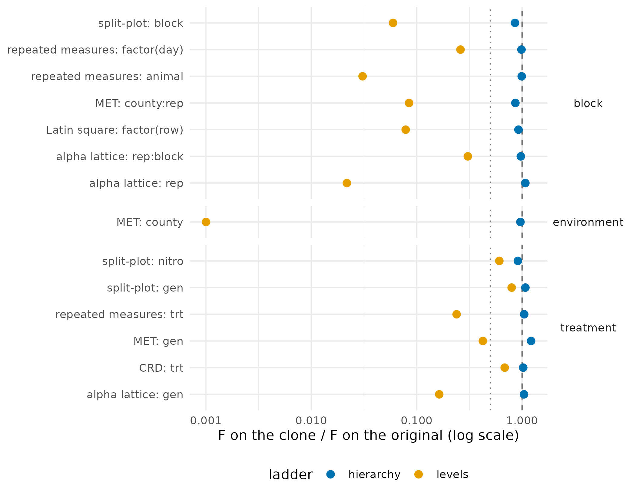
Dot plot of clone-to-original F ratios for every design term, two ladders side by side.

F statistic of each model term on the clone as a share of the original, median over twenty seeds, by ladder. Points on the dashed line are terms the clone reproduces exactly; the dotted line is the pass floor of one half. The levels ladder loses most of every blocking and environment term; the hierarchy ladder keeps them.

Results

All 8 of the 8 designs pass the rule under the hierarchy ladder. The allocation and the NA mask come back identical in every clone of every design, under both ladders. The ladder decides what a model finds.

The multi-environment trial is the case the hierarchy ladder was built for. Its county effect has an F of 987 on the original; the levels ladder drops county before rep, and the clone’s county F is 1. The hierarchy ladder conditions on genotype alone and carries the plot coordinates, county, rep, block and their pairs as shifts. Under it the clone’s county F is 952, and the nested county:rep term is at 28.3 against 32.7. The genotype means correlate at 0.9 with the original, against 0.68 under the levels ladder.

Yates’ oats shows the same thing on a single trial: the block F is 0.8 under the levels ladder and 11.3 under the hierarchy ladder, against 13.2 on the original, while the nitrogen response is kept by both.

The alpha lattice and the RCBD are three-replicate variety trials, and there the treatment-only rung is itself below the floor of five rows: every row is pooled. Under the levels ladder that clone is the marginal clone, with a genotype correlation near zero; under the hierarchy ladder the genotype means are carried as a shift and the correlation is 0.93 on the lattice and 0.89 on the RCBD.

The augmented design is the one where the rule has the least to say: its block and check terms are not detectable on the original (F below 2), so only the allocation, the NA mask and the spread of the treatment means are tested. The clone does not, and cannot, carry the unreplicated entries’ values.

Limits

The rule tests fixed-effects F statistics from lm(). A split-plot or a repeated-measures analysis would normally use a mixed model with the right error strata; the F ratios here compare the same fixed-effects model on both sides and say nothing about variance components. The treatment check compares level means over replicated levels, so it does not see a treatment-by-environment interaction, which the clone does not preserve: the copula is fitted within the stratum the ladder reached, and once county has been dropped the genotype-by-county pattern is gone. What the clone carries of a dropped column is an additive main effect, shrunk toward zero when the column explains little; a spatial trend recorded only as row and column numbers is carried as row and column means, not as a surface. The floors in the rule (half the original F, a correlation of 0.7, a spread within a factor of two) are the tolerances this vignette states, not properties of the method; tighten them and re-run the chunk for a stricter test.

What to read next

Confidentiality and the threat model lists what carrying a level mean into the clone discloses: a level with only a few plots reveals close to its real mean. Getting started with masque is the custodian’s path from a table to a synthetic and a recipe.

Reproduce

set.seed(1) is set once for the document; every mask() call passes its own seed, one to twenty, so each clone is reproducible on its own. Package versions follow.

sessionInfo()
#> R version 4.6.1 (2026-06-24)
#> Platform: x86_64-pc-linux-gnu
#> Running under: Ubuntu 24.04.5 LTS
#> 
#> Matrix products: default
#> BLAS:   /usr/lib/x86_64-linux-gnu/openblas-pthread/libblas.so.3 
#> LAPACK: /usr/lib/x86_64-linux-gnu/openblas-pthread/libopenblasp-r0.3.26.so;  LAPACK version 3.12.0
#> 
#> locale:
#>  [1] LC_CTYPE=C.UTF-8       LC_NUMERIC=C           LC_TIME=C.UTF-8        LC_COLLATE=C.UTF-8    
#>  [5] LC_MONETARY=C.UTF-8    LC_MESSAGES=C.UTF-8    LC_PAPER=C.UTF-8       LC_NAME=C             
#>  [9] LC_ADDRESS=C           LC_TELEPHONE=C         LC_MEASUREMENT=C.UTF-8 LC_IDENTIFICATION=C   
#> 
#> time zone: UTC
#> tzcode source: system (glibc)
#> 
#> attached base packages:
#> [1] stats     graphics  grDevices utils     datasets  methods   base     
#> 
#> other attached packages:
#> [1] masque_0.14.1.9000
#> 
#> loaded via a namespace (and not attached):
#>  [1] vctrs_0.7.3         cli_3.6.6           knitr_1.52          rlang_1.3.0        
#>  [5] xfun_0.61           otel_0.2.0          S7_0.2.2            textshaping_1.0.5  
#>  [9] data.table_1.18.6.1 jsonlite_2.0.0      glue_1.8.1          htmltools_0.5.9    
#> [13] ragg_1.5.2          sass_0.4.10         scales_1.4.0        rmarkdown_2.32     
#> [17] grid_4.6.1          evaluate_1.0.5      jquerylib_0.1.4     fastmap_1.2.0      
#> [21] yaml_2.3.12         lifecycle_1.0.5     compiler_4.6.1      RColorBrewer_1.1-3 
#> [25] fs_2.1.0            farver_2.1.2        systemfonts_1.3.2   digest_0.6.39      
#> [29] R6_2.6.1            bslib_0.12.0        withr_3.0.3         tools_4.6.1        
#> [33] gtable_0.3.6        agridat_1.26        pkgdown_2.2.1       ggplot2_4.0.3      
#> [37] cachem_1.1.0        desc_1.4.3