![[Experimental]](figures/lifecycle-experimental.svg)
Render a pairwise, asymmetric matrix of smoothed associations between
numeric variables. Each cell [i, j] where i != j shows the fitted
spline from mgcv::gam():
Upper triangle (
i < j):gam(x_j ~ s(x_i) + <adjust>).Lower triangle (
i > j):gam(x_i ~ s(x_j) + <adjust>).Diagonal: blank panel when labels live on the border (default), or a variable-name label when
labels = "diagonal".
The two triangles intentionally differ — the asymmetry reveals heteroscedasticity, leverage, and directional non-linearity that a single scalar correlation hides.
Usage
janusplot(
  data,
  vars = NULL,
  adjust = NULL,
  method = NULL,
  k = -1L,
  bs = "tp",
  engine = c("bam", "gam"),
  discrete = FALSE,
  nthreads = 1L,
  order = c("original", "hclust", "alphabetical"),
  show_data = TRUE,
  show_ci = TRUE,
  display = c("fit", "d1", "d2"),
  derivative_ci = c("none", "pointwise", "simultaneous"),
  derivative_ci_nsim = 1000L,
  n_grid = NULL,
  colour_by = c("pearson", "spearman", "kendall", "edf", "deviance_gap", "none"),
  fill_by = NULL,
  palette = NULL,
  annotations = c("edf", "A"),
  shape_cutoffs = janusplot_shape_cutoffs(),
  show_shape_legend = TRUE,
  glyph_style = c("ascii", "unicode"),
  labels = c("border", "diagonal", "none"),
  diagonal = c("auto", "blank", "name", "density"),
  label_srt = 45,
  label_cex = 1,
  signif_glyph = TRUE,
  show_asymmetry = NULL,
  na_action = c("pairwise", "complete"),
  parallel = FALSE,
  with_data = FALSE,
  text_scale_diag = 1,
  text_scale_off_diag = 1,
  show_glossary = TRUE,
  glossary_scale = 1,
  k_check_thresholds = NULL,
  auto_refit_k = FALSE,
  k_max_iter = 2L,
  compact = c("auto", "always", "never"),
  compact_threshold = 12L,
  compact_levels = NULL,
  focus_by = NA_character_,
  focus_threshold = "q90",
  focus_dim_alpha = 0.25,
  axes = c("original", "standardised", "centred", "rank"),
  save_as = NULL,
  save_width = NULL,
  save_height = NULL,
  save_dpi = 300,
  ...
)
Arguments
- data
A data frame with numeric columns to include.
- vars
Character vector of column names to use.
NULL(default) uses all numeric columns indata. Non-numeric columns trigger an error listing offenders.- adjust
A one-sided formula RHS giving additional covariates and/or random effects to include in every pairwise GAM. For example,
adjust = ~ s(age) + s(site, bs = "re")fitsgam(y ~ s(x) + s(age) + s(site, bs = "re"))for each pair. DefaultNULLfits unadjusted pairwise smooths.- method
Smoothing-parameter estimation method passed to the chosen fitting backend. Default
NULLresolves per-engine:"fREML"forengine = "bam"(mgcv's recommended at scale),"REML"forengine = "gam"(the v0.1.0 behaviour). Pass any valid mgcv method string to override.- k
Integer, or named list mapping variable names to integers. Basis dimension for
s(). Default-1L(mgcv's automatic choice).- bs
Basis type for
s(). Default"tp"(thin plate).- engine
One of
"bam"(default, new in v0.1.1) or"gam". Selects mgcv's fitting backend:"bam"—mgcv::bam(). Block-Lanczos solve + fREML estimation + lower memory. ~3-10x speedup at janusplot's scale (k = 15-25 vars, 600+ pairwise fits per call). The default, and the one non-byte-identical change in v0.1.1: fREML differs from REML by ~1-3% in EDF on identical data, so the asymmetry index may shift by similar amounts vs v0.1.0 output. Recoverable verbatim viaengine = "gam"."gam"—mgcv::gam(). The v0.1.0 backend. Use for backward-compat reproduction, very small n (< 200) where bam's setup overhead exceeds its solve gain, or methodologically sensitive contexts that require REML rather than fREML.
- discrete
Logical.
bam-only opt-in to mgcv's covariate-discretisation optimisation. Further ~2-5x speedup at the cost of small (sub-pixel at typical janusplot resolution) prediction-shift. DefaultFALSE. Ignored whenengine = "gam".- nthreads
Integer.
bam-only intra-fit threading. Default1Lto avoid oversubscription when combined withparallel = TRUE(future.applyfans out pair fits across cores; nthreads > 1 within each pair would double-book CPUs). Raise above 1 only whenparallel = FALSE. Ignored whenengine = "gam".- order
One of
"original"(default),"hclust"(reorder by hierarchical clustering of Pearson correlations), or"alphabetical".- show_data
Logical. If
TRUE(default), overlay raw data points (low alpha) behind each spline. Only applies whendisplay = "fit"; derivative panels never overlay raw data.- show_ci
Logical. If
TRUE(default), overlay the 95% confidence envelope frompredict(gam, se.fit = TRUE)on the fit panel (i.e. whendisplay = "fit"). CI rendering on derivative panels is controlled separately byderivative_ci.- display
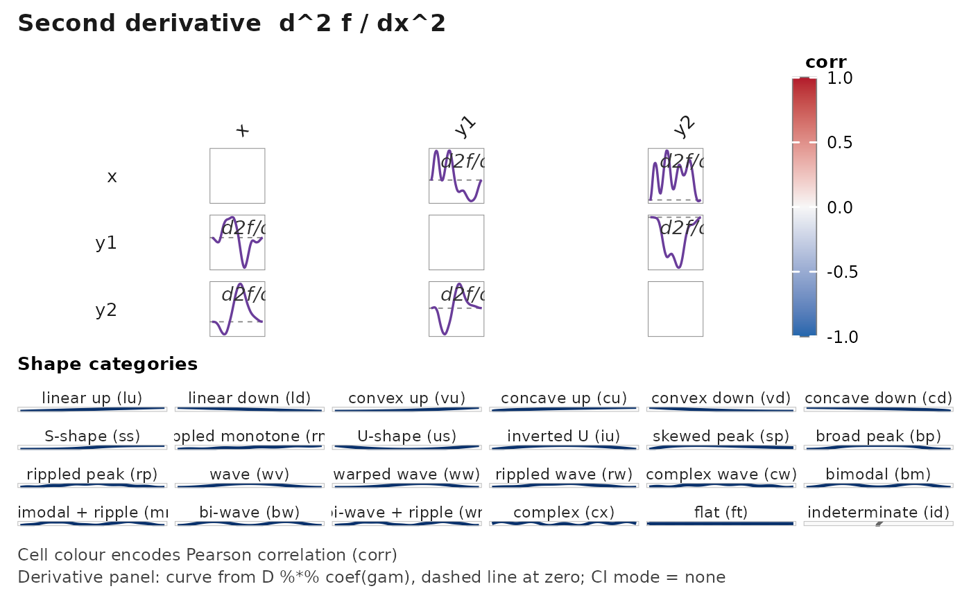
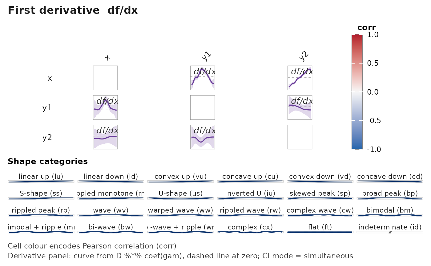
One of
"fit"(default),"d1", or"d2". Selects which single quantity is rendered in every off-diagonal cell of the matrix."fit"— the fitted smooth \(\hat f(x)\); default, behaviour identical to the pre-derivative release."d1"— the first derivative \(\hat f'(x)\) of the fitted smooth. Zero crossings localise turning points of \(\hat f\)."d2"— the second derivative \(\hat f''(x)\). Zero crossings localise inflection points of \(\hat f\).
A single matrix shows a single quantity by design: stacked multi-panel cells crowd the matrix at any realistic variable count. To compare fit against derivative, render two or three
janusplot()calls side-by-side; each call keeps its ownwith_data = TRUEsummary table tagged with thedisplaycolumn.Orders \(k \ge 3\) are not exposed — higher-order derivatives of penalised regression splines amplify noise and rarely carry usable signal at realistic sample sizes. See
vignette("janusplot")for the theoretical justification and applied use-cases.- derivative_ci
One of
"none"(default),"pointwise", or"simultaneous". Controls whether — and how — a 95% confidence ribbon is drawn underneath the derivative curve whendisplay %in% c("d1", "d2"). Ignored whendisplay = "fit"."none"— no ribbon. The curve and the zero reference line are all you see. Default, because pointwise ribbons overshoot nominal coverage as a joint region and can invite over-reading of local features."pointwise"— 95% pointwise ribbon from \(\sqrt{\mathrm{diag}(D V_p D^\top)}\) (Wood 2017 §7.2.4). Valid marginally; not a simultaneous statement."simultaneous"— 95% simultaneous band via the Monte Carlo construction of Ruppert, Wand & Carroll (2003) popularised for GAMs by Simpson (2018, Frontiers Ecol. Evol. 6:149): draw \(B\) samples \(\tilde{\boldsymbol\beta} \sim \mathcal{N}(\hat{\boldsymbol\beta}, V_p)\), compute \(\max_x |D_i(\tilde{\boldsymbol\beta} - \hat{\boldsymbol\beta})| / \mathrm{se}_i\), and use the \((1-\alpha)\) quantile as a critical multiplier on the pointwise SE. Valid for feature localisation ("where is \(\hat f'(x)\) significantly non-zero").
- derivative_ci_nsim
Integer. Number of Monte Carlo samples used when
derivative_ci = "simultaneous". Default1000L— a compromise between coverage accuracy (Simpson 2018 uses 10000) and CPU budget across every pair in a medium-sized matrix. Ignored for any otherderivative_ci.- n_grid
Integer or
NULL. Number of equally-spaced points used to evaluate each fitted smooth (and its derivatives). DefaultNULLresolves to100whendisplay = "fit"and200otherwise, because finite-difference second derivatives visibly degrade below \(\sim 150\) points on moderate-ksmooths. Supplyingn_griddirectly overrides both defaults. Larger grids shift the numerical shape-metric values (\(M\), \(C\), turning / inflection counts) slightly because they are computed on this same grid. Shapes and asymmetry are the primary reading;M,Cand the counts are secondary diagnostics and the grid-induced drift is tolerable.- colour_by
One of
"pearson"(default),"spearman","kendall","edf","deviance_gap", or"none". Encodes the per-cell fill colour by the chosen scalar. Correlation choices use a diverging palette with limitsc(-1, 1)and a sharedcorrcolour-bar title;"edf"and"deviance_gap"use a sequential palette labelled by the metric.- fill_by
Deprecated alias for
colour_by. If supplied emits a single soft deprecation warning and is forwarded tocolour_by.- palette
Character. Colour palette for the cell fill scale. Defaults to
"RdBu"whencolour_byis a correlation and"viridis"otherwise. Sequential choices:"viridis","magma","inferno","plasma","cividis","mako","rocket","turbo"(not CB-safe),"YlOrRd","YlGnBu","Blues","Greens". Diverging choices:"RdYlBu","RdBu","PuOr","Spectral"(not CB-safe). Passing a sequential palette whilecolour_byis a correlation silently upgrades to the default diverging palette.- annotations
Character vector, a subset of
c("edf", "A", "shape", "code"). Controls which corner annotations appear on each off-diagonal cell:"code"— 2-letter ASCII shape code, top-left corner."A"and"edf"— asymmetry index and effective degrees of freedom, stacked bottom-left."shape"— shape glyph (Unicode or ASCII perglyph_style), bottom-right corner.
Default
c("edf", "A")."code"and"shape"occupy distinct corners so both can be requested together. Seejanusplot_shape_hierarchy()for the full code list.- shape_cutoffs
Named list of classification thresholds used to map the continuous shape indices into discrete
shape_categorylabels; seejanusplot_shape_cutoffs().- show_shape_legend
Logical. If
TRUE(default), attach a standing shape-types legend plate below the matrix that illustrates every category in the taxonomy as a canonical thumbnail spline. Independent ofannotations.- glyph_style
One of
"ascii"(default) or"unicode". Controls how cell shape glyphs render when"shape"is included inannotations. Default is"ascii"for maximum portability across typesetting pipelines; switch to"unicode"only when the target font is known to cover the curve glyph set.- labels
One of
"border"(default),"diagonal", or"none". Controls where variable names are rendered:"border"— names along the top (rotated perlabel_srt) and left margins of the matrix; diagonal cells are left blank. Mirrorscorrplot'stl.pos = "lt"convention."diagonal"— names centred on the diagonal cells (the pre-0.1 layout)."none"— labels suppressed entirely; diagonal cells blank.
- diagonal
One of
"auto"(default),"blank","name", or"density". Controls what is rendered in the diagonal cells of the matrix."auto"— preserves the historical behaviour: variable name whenlabels = "diagonal", blank otherwise."blank"— empty bordered panel (uniform grid reading)."name"— variable name centred in the cell, bold."density"— kernel density of the variable filled in translucent grey, with a rug of raw values along the bottom edge. Mirrors theGGally::ggpairsconvention; surfaces tail weight, bimodality, and support clipping that the pairwise smooths alone cannot reveal. Variable names should come from the border (labels = "border", the default) when this mode is on.
- label_srt
Numeric. Rotation (degrees) of top labels when
labels = "border". Default45; set to0for horizontal or90for vertical. Ignored whenlabels != "border".- label_cex
Positive numeric multiplier on the border-label font size. Default
1. Ignored whenlabels = "none".- signif_glyph
Logical. If
TRUE(default), annotate cells with·/*/**reflecting the smooth's F-test p-value.- show_asymmetry
Deprecated. Use
annotationsinstead ("A" %in% annotations). When supplied, a soft deprecation warning fires and the argument is merged intoannotations.- na_action
One of
"pairwise"(default; per-cell complete observations) or"complete"(listwise; all cells use the same rows).- parallel
Logical. If
TRUE, usefuture.apply::future_mapply()to fit pairs in parallel. Requires thefuture.applypackage and a user-configuredfuture::plan(). DefaultFALSE.- with_data
Logical. If
TRUE, return a two-element listlist(plot, data)wheredatais a flat per-cell summary (one row per off-diagonal cell) of everything the plot displays. Thedataelement is always a plaindata.frame(base R — nodata.tabledependency). DefaultFALSE— in which case only the ggplot is returned.- text_scale_diag
Positive numeric multiplier applied to the diagonal variable-name labels. Default
1. Diagonal labels additionally auto-shrink for long variable names (nchar(var) > 10) so they fit the cell regardless of this value.- text_scale_off_diag
Positive numeric multiplier applied to all off-diagonal annotations (
n/EDFreadouts, significance glyphs, asymmetry-index labels). Default1. Use< 1when cells are small and the annotations crowd the fit line; use> 1for presentation plots.- show_glossary
Logical. If
TRUE(default), attach a multi-line caption below the matrix describing the on-plot abbreviations (n,EDF,A, fill encoding, significance glyphs). Only keys actually displayed are listed.- glossary_scale
Positive numeric multiplier on the glossary caption font size. Default
1.- k_check_thresholds
Named list giving the three flag-criterion thresholds used by
mgcv::k.check()-style basis-dimension diagnostics. Required entries:edf_ratio(Wood's \(\widehat{\mathrm{edf}}/k'\) ratio above which the smooth is too close to its basis cap),k_index(residual-difference variance ratio below which the basis appears underspecified), andp(the simulation p-value below which the basis-deficiency signal is significant). Defaults —edf_ratio = 0.9,k_index = 1.0,p = 0.05— trackmgcv::gam.check()and Wood (2017) §5.9.- auto_refit_k
Logical. If
TRUE, every cell whose Wood trifecta flags an underfit is refit with a doubling-k loop until either the flag clears, the per-cell unique-x cap is reached, ork_max_iteriterations have passed. DefaultFALSE— the diagnostic (k_check_status,k_flag,k_prime,k_index,k_p) is always computed and surfaced regardless of this flag, but the refit is opt-in because it can multiply wall time on pathological data.- k_max_iter
Integer. Maximum number of doublings allowed per cell when
auto_refit_k = TRUE. Default2L(so a cell that starts at themgcvdefaultk = 10will visit at mostk = 20and thenk = 40, capped by the per-cell unique-x limit). Ignored whenauto_refit_k = FALSE.- compact
One of
"auto"(default),"always", or"never". Controls scale-aware content suppression per cell:"auto"— tier 0 atn_var < compact_threshold(the v0.1.0 behaviour); progressively suppresses scatter, then CI, then annotations, then the spline itself asn_varcrosses thecompact_levelsladder. The matrix remains readable askgrows toward 25–30 by trading detail for legibility."always"— force at least tier 1 regardless ofn_var. Useful for very dense fixed-size renders."never"— force tier 0 regardless ofn_var. Useful for reproducing v0.1.0 figures on large matrices.
- compact_threshold
Integer. The
n_varvalue at which tier 1 (drop scatter) auto-activates undercompact = "auto". Default12L, anchored on the 150 × 150 px-per-cell pixel budget at typical 6"×6" 300 DPI R Journal figures.- compact_levels
Optional named list with entries
t1,t2,t3overriding the auto-tier ladder. Defaults derive fromcompact_threshold:t1 = compact_threshold,t2 = compact_threshold + 6,t3 = compact_threshold + 13.NULL(default) uses these derived defaults.- focus_by
One of
NA(default — no filter),"asymmetry","edf","k_flag", or"non_linearity"(defined asedf - 1). When set, cells whose chosen metric falls belowfocus_thresholdare rendered ingrey85at alphafocus_dim_alpha; the matrix shape is preserved so attention drains visually to high-metric cells. This is a visual filter, not a statistical one — the underlying fits are unchanged and thewith_datatable carries every cell.- focus_threshold
Either a quantile-string like
"q90"(default) or a numeric cutoff. The quantile is taken over the non-NAdistribution offocus_byacross all off-diagonal cells in the matrix. Ignored whenfocus_by = NA.- focus_dim_alpha
Numeric in
[0, 1]. Alpha applied to thegrey85wash on unfocused cells. Default0.25. Ignored whenfocus_by = NA.- axes
One of
"original"(default),"standardised","centred", or"rank". Rendering-only knob — the underlyingmgcv::gamfits are byte-identical across all four modes (verifiable viadigest::digest()on the fit list); the transformation lives entirely inside the cell renderer and propagates to (a) the raw scatter, (b) the spline prediction grid, (c) the CI ribbon, and (d) the variable label on the matrix border. Use:"original"— raw units. Maximum interpretability per cell. v0.1.0 behaviour."standardised"—(x - mean(x)) / sd(x)per variable. Border label becomes e.g."mpg (z)". Pairs scaled into a comparable visual range; useful atk >= 15when raw-unit panels look disparate."centred"—x - mean(x)per variable. Border label becomes e.g."mpg (centred)". Preserves units while anchoring the origin."rank"— empirical-CDF-based rank, scaled to[0, n]per variable. Border label becomes"rank(mpg)". Sanity-check view: collapses outliers; if the smooth changes shape vs"original"the relationship is monotone-but-not-linear.
At compact tier 3 (
n_var >= 25undercompact = "auto"), the cells render only colour fill + shape-class glyph — no curve, no scatter — soaxesbecomes a documented no-op (the border labels still pick up the mode suffix).- save_as
Optional file path with extension. When set, the final assembled plot is written to this path via
ggplot2::ggsave(); the device is inferred from the extension. Supported extensions:.png,.pdf,.svg,.jpg/.jpeg,.tif/.tiff,.eps,.ps,.bmp. DefaultNULL(no file written;janusplot()still returns the ggplot). Width / height default topmax(6, 0.65 * k_n)inches each — square aspect, scaling with matrix dimension.- save_width
Numeric. Override width (inches) for
save_as. DefaultNULLuses the auto-resolved square.- save_height
Numeric. Override height (inches) for
save_as. DefaultNULLuses the auto-resolved square.- save_dpi
Integer. Raster DPI for
save_aswhen the inferred device is bitmap (png/jpg/tiff/bmp). Default300, matching the R Journal target.- ...
Additional arguments passed to
mgcv::gam().
Value
If with_data = FALSE (default), a ggplot2::ggplot object
(via patchwork::wrap_plots()) carrying a top-of-matrix title
that names the displayed quantity ("Direct fit",
"First derivative f'", or "Second derivative f''"). If
with_data = TRUE, a list with two elements: plot (the
ggplot) and data (a tidy table with columns var_x, var_y,
position, n_used, edf, pvalue, signif, dev_exp,
asymmetry_index, cor_pearson, cor_spearman,
cor_kendall, tie_ratio, monotonicity_index,
convexity_index, n_turning_points, n_inflections,
flat_range_ratio, shape_category, colour_value,
display, one row per off-diagonal cell). The display
column tags which quantity the call rendered, so separate
calls for fit / d1 / d2 yield comparable, stackable tables.
Derivative curves themselves (grid of \(x\), fitted
\(\hat f^{(k)}\), SE) live on janusplot_data() — see there.
See also
janusplot_data() for the raw per-cell fits + metrics.
Other smooth-associations:
janusplot_data()
Examples
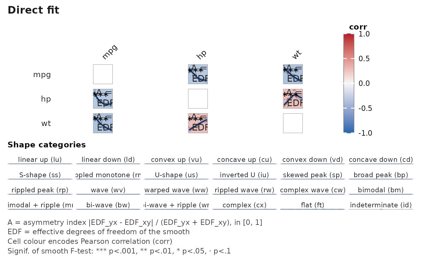
# Minimal runnable example — 3 variables, 6 asymmetric pairwise GAM fits.
janusplot(mtcars[, c("mpg", "hp", "wt")])
 # \donttest{
# Heteroscedastic DGP: Pearson r is ~ 0.9 but the inverse fit is
# clearly non-linear, yielding asymmetry index > 0.5.
set.seed(2026L)
n <- 200L
x1 <- stats::runif(n, 0, 10)
x2 <- x1 + stats::rnorm(n, sd = 0.2 * x1)
janusplot(data.frame(x1 = x1, x2 = x2, x3 = stats::rnorm(n)))
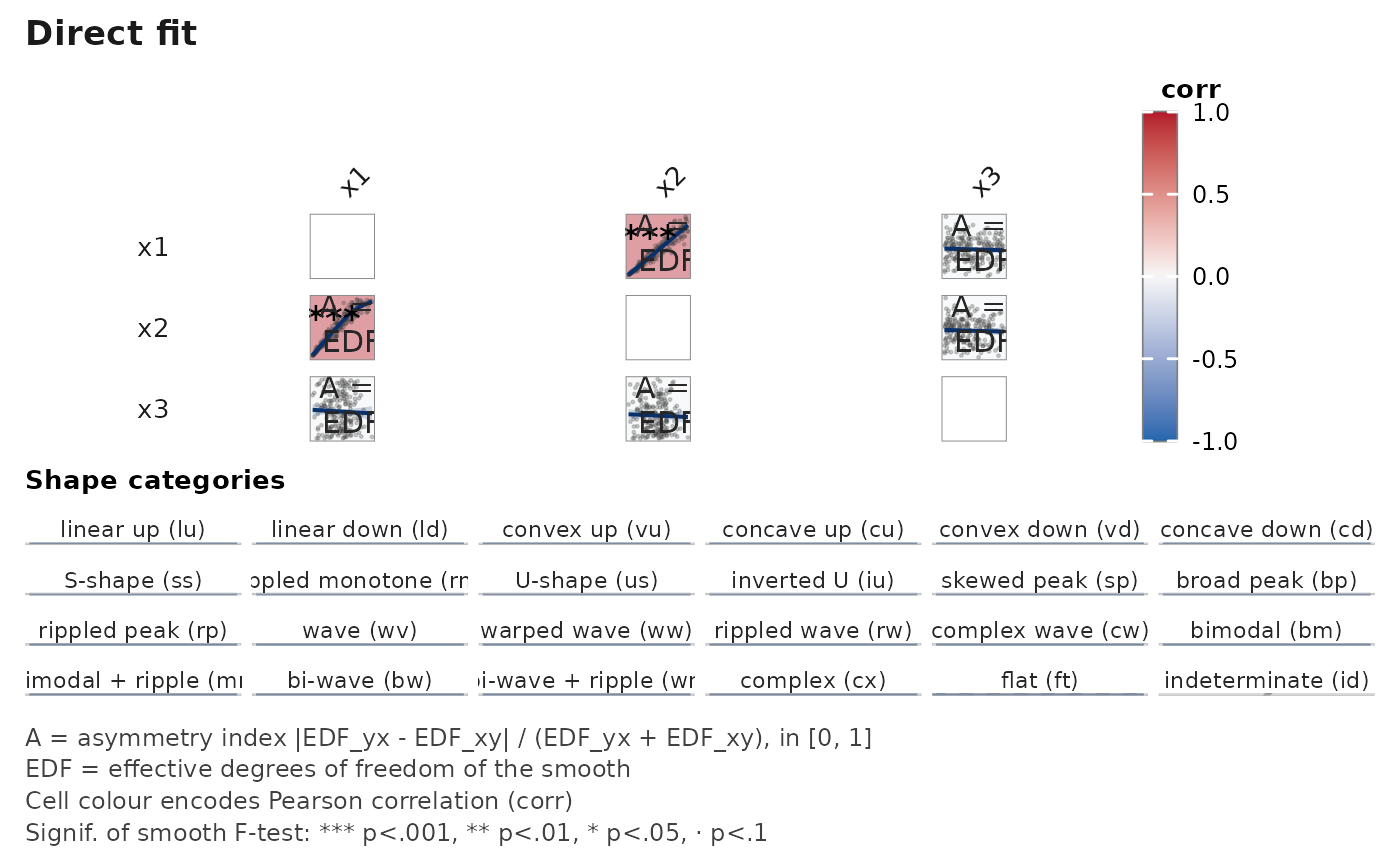
# \donttest{
# Heteroscedastic DGP: Pearson r is ~ 0.9 but the inverse fit is
# clearly non-linear, yielding asymmetry index > 0.5.
set.seed(2026L)
n <- 200L
x1 <- stats::runif(n, 0, 10)
x2 <- x1 + stats::rnorm(n, sd = 0.2 * x1)
janusplot(data.frame(x1 = x1, x2 = x2, x3 = stats::rnorm(n)))
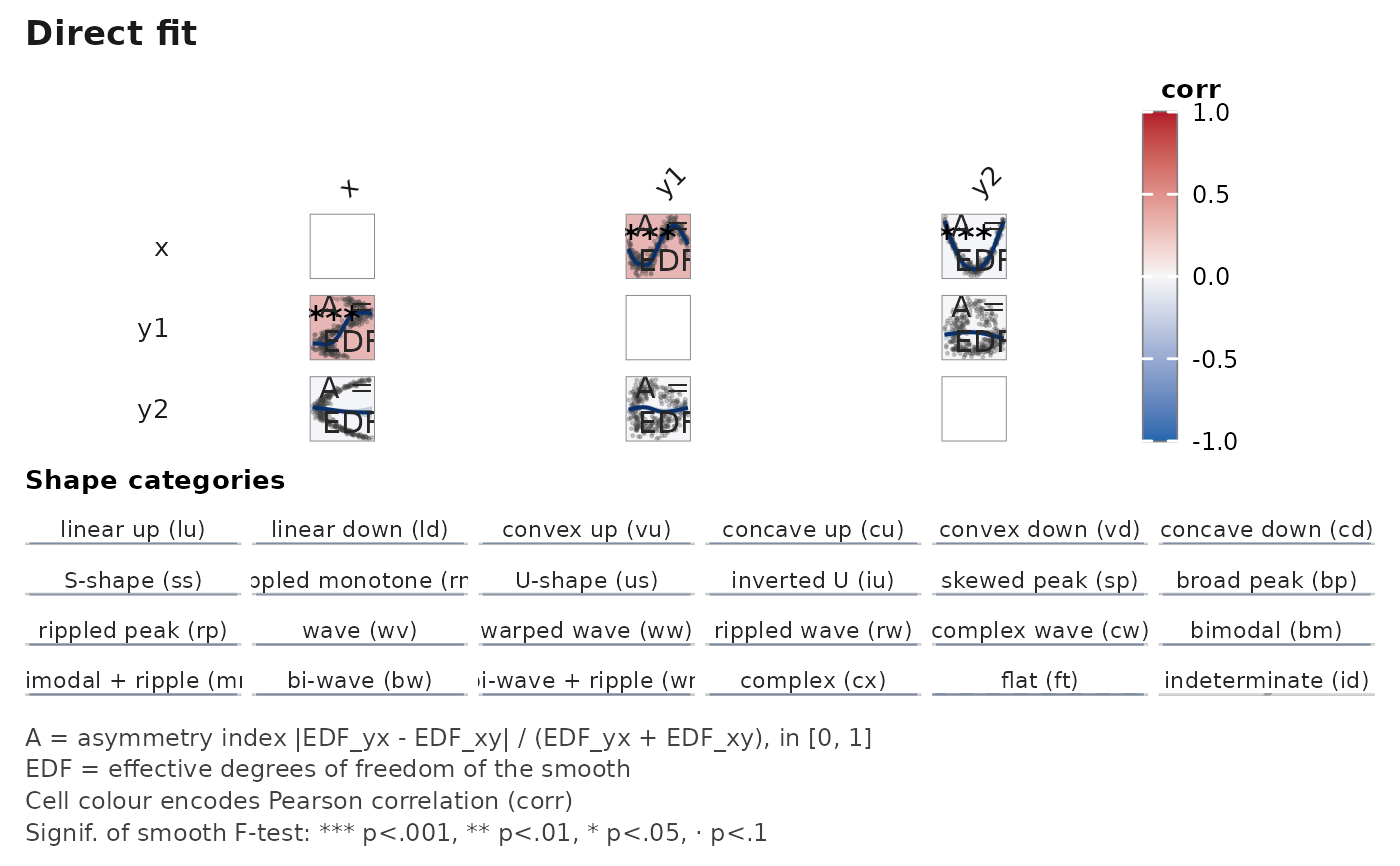
 # A single matrix renders a single quantity. To compare the fit
# against its derivatives, render three calls and place them
# side-by-side; each call's title makes the quantity explicit.
set.seed(2026L)
xs <- stats::runif(300L, -3, 3)
df <- data.frame(
x = xs,
y1 = sin(xs) + stats::rnorm(300L, sd = 0.3),
y2 = xs^2 + stats::rnorm(300L, sd = 0.6)
)
janusplot(df, display = "fit")
# A single matrix renders a single quantity. To compare the fit
# against its derivatives, render three calls and place them
# side-by-side; each call's title makes the quantity explicit.
set.seed(2026L)
xs <- stats::runif(300L, -3, 3)
df <- data.frame(
x = xs,
y1 = sin(xs) + stats::rnorm(300L, sd = 0.3),
y2 = xs^2 + stats::rnorm(300L, sd = 0.6)
)
janusplot(df, display = "fit")
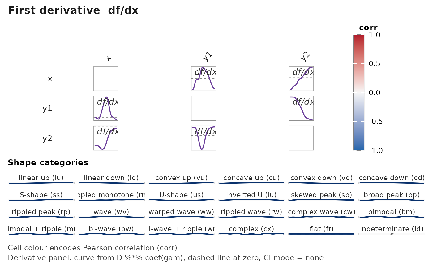
 janusplot(df, display = "d1")
 janusplot(df, display = "d2")
 # Simultaneous CI bands on a derivative panel, per Simpson (2018).
janusplot(df, display = "d1", derivative_ci = "simultaneous")
# Simultaneous CI bands on a derivative panel, per Simpson (2018).
janusplot(df, display = "d1", derivative_ci = "simultaneous")
 # }
# }