Which parameters change the shape of the output distribution? • kernR

library(kernR)

Why

A risk modeller is ranking the parameters of a crop model and does not trust the ranking. The variance budget says one parameter dominates and the rest are negligible. But two of those negligible parameters are the ones that decide whether a bad season is merely poor or a write-off: one fattens the lower tail and one skews the whole distribution, neither of them changes the variance much. Is there a sensitivity index that ranks a parameter by what it does to the distribution rather than by how much variance it explains? This vignette answers with the HSIC-based sensitivity index, on a synthetic simulator whose parameters were built to separate the two questions, and then adds total-order indices for the parameters that act only in combination.

What

A variance-based Sobol index decomposes the output variance into contributions from each input, which makes it blind by construction to any effect that leaves the variance where it was. The HSIC-Sensitivity Index of Da Veiga (2015) replaces the variance with a kernel dependence measure. The normalised first-order index is

$S_j^{\mathrm{HSIC}} = \frac{\mathrm{HSIC}(X_j, Y)} {\sqrt{\mathrm{HSIC}(X_j, X_j) \cdot \mathrm{HSIC}(Y, Y)}} \in [0, 1],$

bounded like a Sobol index, comparable across parameters, and sensitive to any change in the conditional distribution of the output, including the mean-preserving ones.

hsic_sensitivity() computes it for every parameter against every output, with a permutation p-value per pair and a Benjamini-Hochberg adjustment across the grid. total_order = TRUE adds the total-order index in Da Veiga’s complement form,

$T_j^{\mathrm{HSIC}} = 1 - \frac{\mathrm{HSIC}(X_{\sim j}, Y)} {\sqrt{\mathrm{HSIC}(X_{\sim j}, X_{\sim j}) \cdot \mathrm{HSIC}(Y, Y)}},$

which measures the contribution of $X_j$ directly plus through every interaction it takes part in. total_order_ci = TRUE attaches a pair-bootstrap percentile interval to each total-order index, and total_order_test = "cond_perm" attaches a conditional-permutation significance test to it. lhs_design() builds the design; plot() and as.data.frame() render the result.

Do

A simulator built to separate the two questions

A synthetic stub with four parameters, each carrying one kind of effect. mean_effect shifts the mean, which a variance budget also sees. var_effect changes the spread and nothing else. tail_effect injects a heavy-tailed component, changing the shape without moving the centre. inert does nothing.

stub_apsim <- function(theta) {
  n_row <- nrow(theta)
  yield <- 1.5 * theta[, "mean_effect"] +
    rnorm(n_row, sd = exp(theta[, "var_effect"])) +
    theta[, "tail_effect"] * rt(n_row, df = 3) * 0.4 +
    rnorm(n_row, sd = 0.05)
  matrix(yield, ncol = 1L, dimnames = list(NULL, "yield"))
}

set.seed(1L)
bounds <- rbind(
  mean_effect = c(0.0, 1.0),
  var_effect  = c(-0.5, 0.5),
  tail_effect = c(0.0, 1.0),
  inert       = c(0.0, 1.0)
)
design <- lhs_design(n = 600L, bounds = bounds, seed = 11L)
yield <- stub_apsim(design)

The first-order scan

fit <- hsic_sensitivity(
  theta = design, y = yield, n_permutations = 199L, seed = 11L
)
fit
#> 
#>   HSIC-Sensitivity Indices
#> 
#> Parameters:   4 
#> Outputs:      1 
#> N:            600 
#> Permutations: 199 
#> P-adjust:     BH 
#> Total-order: no
#> 
#> Per-parameter ranking (descending S, max across outputs):
#>   S = first-order index
#> 
#>    parameter S_first_max min_p_first
#>  mean_effect       0.101      0.0100
#>   var_effect       0.067      0.0100
#>  tail_effect       0.009      0.0600
#>        inert       0.001      0.9450

First-order HSIC-Sensitivity Indices on the 600-row design, ranked, with p-values adjusted by BH.
Parameter	Output	Index	HSIC statistic	p-value	Adjusted p-value
mean_effect	yield	0.1009	0.00840	0.005	0.010
var_effect	yield	0.0671	0.00559	0.005	0.010
tail_effect	yield	0.0090	0.00075	0.045	0.060
inert	yield	0.0013	0.00011	0.945	0.945

plot(fit)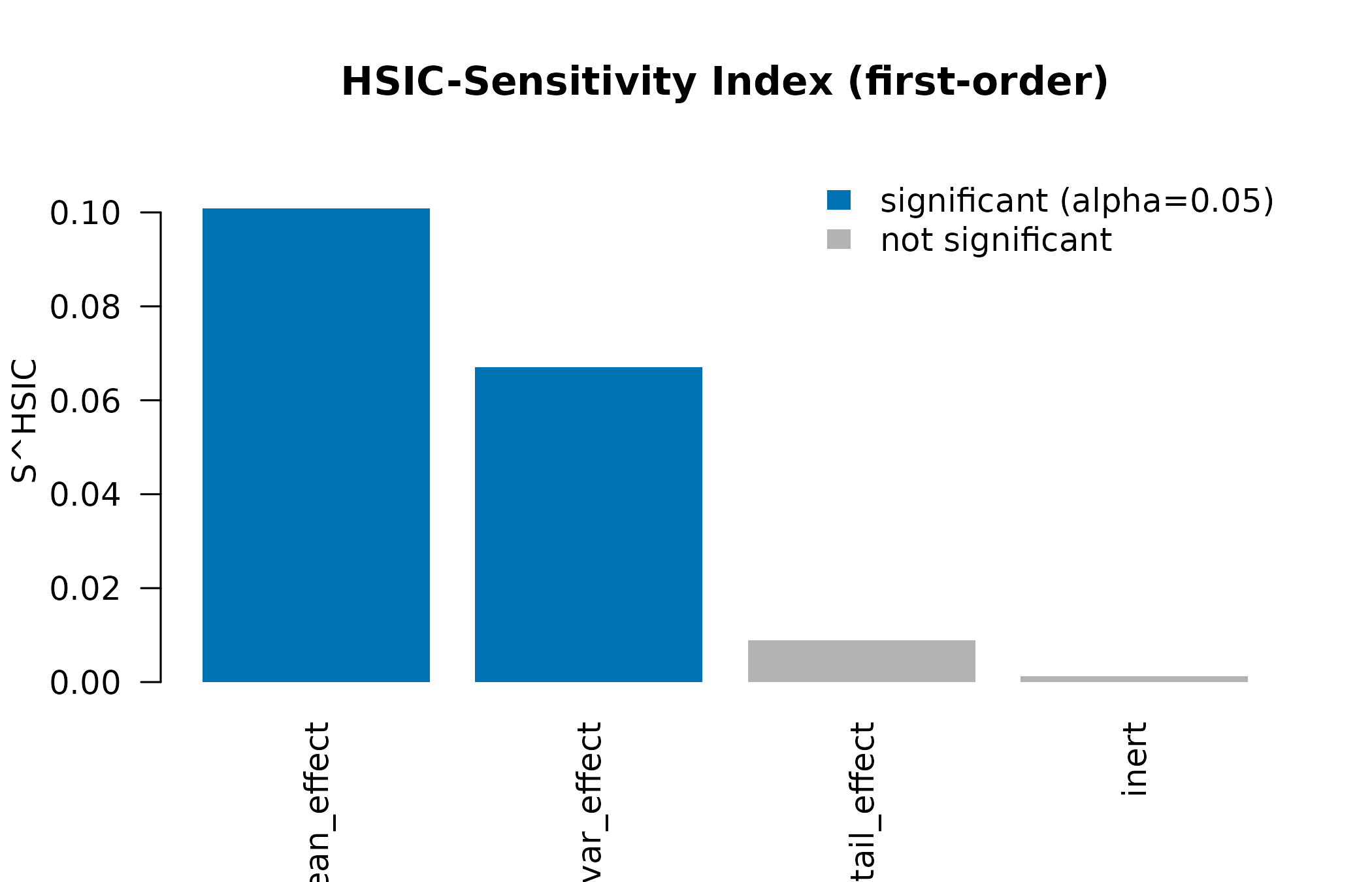

The package’s own diagnostic: first-order HSIC-Sensitivity Index per parameter, bars coloured by significance after Benjamini-Hochberg adjustment at alpha = 0.05.

The figure: the distributions behind the index

halves <- do.call(rbind, lapply(colnames(design), function(p1) {
  data.frame(
    parameter = p1,
    half = ifelse(design[, p1] > median(design[, p1]),
                  "upper half of range", "lower half of range"),
    yield = yield[, "yield"],
    stringsAsFactors = FALSE
  )
}))
ggplot2::ggplot(halves, ggplot2::aes(x = yield, fill = half)) +
  ggplot2::geom_density(alpha = 0.55, colour = NA) +
  ggplot2::facet_wrap(~parameter) +
  ggplot2::scale_fill_viridis_d(name = NULL, end = 0.8) +
  ggplot2::labs(
    x = "yield (arbitrary units)", y = "density",
    title = "What each parameter does to the output distribution"
  ) +
  ggplot2::theme_minimal() +
  ggplot2::theme(legend.position = "bottom")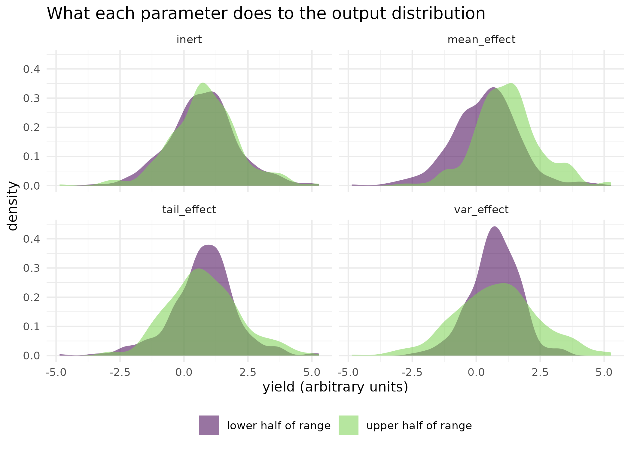

The yield distribution when each parameter is in the lower half of its range against the upper half, one panel per parameter. Under mean_effect the curve slides sideways, which a variance budget also detects. Under var_effect and tail_effect the curve changes width and weight while staying where it is, which is the effect a variance budget is blind to. Under inert the two curves lie on top of each other.

Comparing against Sobol

The sensitivity package is not a dependency of kernR, so the comparison below is shown as code rather than run here. The expected contrast is that a variance-based index ranks mean_effect first and returns small first-order indices for var_effect and tail_effect, because neither moves the output variance far.

half <- nrow(design) / 2
sobol_fit <- sensitivity::sobolEff(
  model = function(X) stub_apsim(as.matrix(X))[, 1L],
  X1    = as.data.frame(design[seq_len(half), ]),
  X2    = as.data.frame(design[seq_len(half) + half, ]),
  nboot = 200
)
# compare sobol_fit$S against fit$index

The disagreement is the point. When the HSIC index ranks a variance-flat parameter highly, that parameter is changing the output distribution in a way the variance budget cannot express.

Total-order indices, and a pure interaction

The first-order index measures what a parameter does on its own. It misses a parameter that acts only through an interaction, and the total-order index is built for exactly that case. The synthetic design below is the extreme version: the output is the product of two parameters, so each has a marginal expectation of zero and neither matters alone.

set.seed(42L)
n_int <- 400L
theta_int <- matrix(
  runif(n_int * 2L, min = -1, max = 1), n_int, 2L,
  dimnames = list(NULL, c("x1", "x2"))
)
y_int <- theta_int[, "x1"] * theta_int[, "x2"] + rnorm(n_int, sd = 0.05)

fit_int <- hsic_sensitivity(
  theta = theta_int, y = y_int, total_order = TRUE,
  p_value = FALSE, n_permutations = 199L, seed = 42L
)
fit_int
#> 
#>   HSIC-Sensitivity Indices
#> 
#> Parameters:   2 
#> Outputs:      1 
#> N:            400 
#> Permutations: skipped (p_value = FALSE)
#> Total-order: yes
#> 
#> Per-parameter ranking (descending S, max across outputs):
#>   S = first-order index   T = total-order index   interaction = T - S
#> 
#>  parameter S_first_max T_total_max interaction min_p_first
#>         x1       0.100       0.906       0.806          --
#>         x2       0.094       0.900       0.806          --

plot(fit_int, which = "both")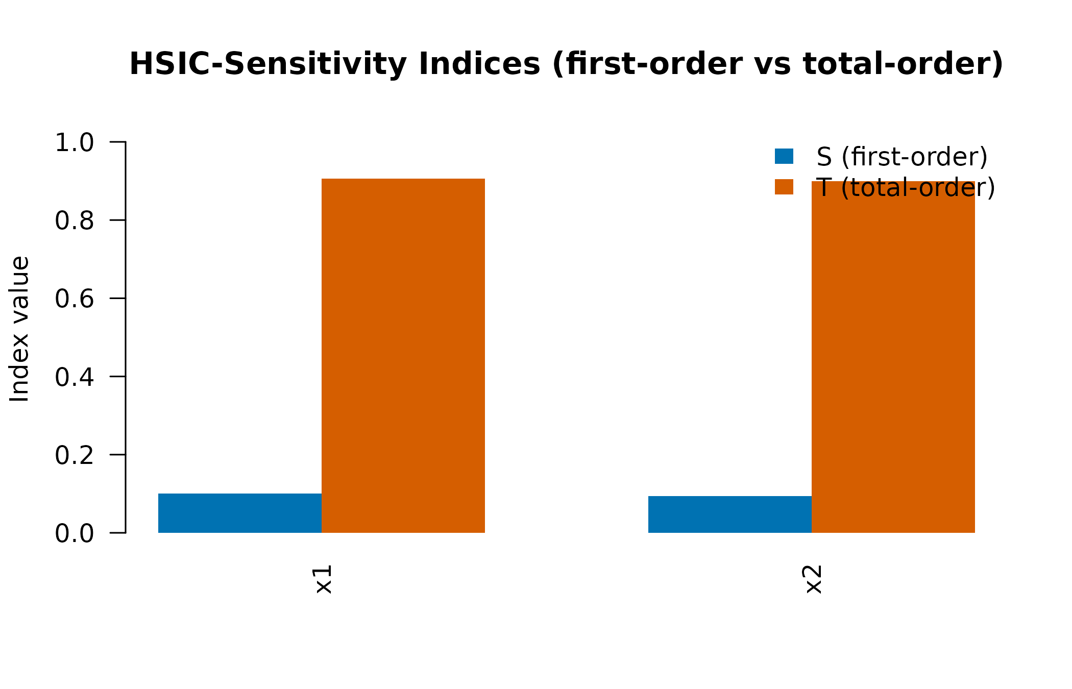

The package’s own diagnostic: first-order against total-order HSIC-Sensitivity Index for x1 and x2 on the pure-interaction model, side by side. The gap between the two bars is the interaction screen in graphical form.

A near-additive design for contrast

theta_add <- matrix(
  runif(n_int * 2L), n_int, 2L, dimnames = list(NULL, c("x1", "x2"))
)
y_add <- 2 * theta_add[, "x1"] + theta_add[, "x2"] +
  rnorm(n_int, sd = 0.05)

fit_add <- hsic_sensitivity(
  theta_add, y_add, total_order = TRUE, p_value = FALSE, seed = 1L
)
fit_add
#> 
#>   HSIC-Sensitivity Indices
#> 
#> Parameters:   2 
#> Outputs:      1 
#> N:            400 
#> Permutations: skipped (p_value = FALSE)
#> Total-order: yes
#> 
#> Per-parameter ranking (descending S, max across outputs):
#>   S = first-order index   T = total-order index   interaction = T - S
#> 
#>  parameter S_first_max T_total_max interaction min_p_first
#>         x1       0.721       0.884       0.163          --
#>         x2       0.116       0.279       0.163          --

First-order and total-order indices on the pure-interaction and near-additive designs, both with 400 design rows.
Design	Parameter	First-order S	Total-order T	T minus S
interaction, Y = X1 X2	x1	0.100	0.906	0.806
interaction, Y = X1 X2	x2	0.094	0.900	0.806
additive, Y = 2 X1 + X2	x1	0.721	0.884	0.163
additive, Y = 2 X1 + X2	x2	0.116	0.279	0.163

An interval on the total-order index

total_order_ci = TRUE attaches a pair-bootstrap percentile interval to each total-order index. It quantifies uncertainty in the magnitude of the index; it is not a hypothesis test.

fit_ci <- hsic_sensitivity(
  theta_add, y_add, total_order = TRUE, total_order_ci = TRUE,
  n_permutations = 199L, n_bootstrap = 100L, ci_level = 0.95, seed = 7L
)
ci_df <- as.data.frame(fit_ci)[, c(
  "parameter", "output", "index_total_order",
  "ci_total_order_lower", "ci_total_order_upper"
)]

Pair-bootstrap percentile interval on each total-order index, 95 per cent level, 100 resamples.
Parameter	Output	Total-order T	Lower	Upper
x1	y1	0.884	0.836	0.920
x2	y1	0.279	0.242	0.322

An earlier release attached a total_order_p_value to these bootstrap draws, claiming to test $H_0 : T_j = 0$ . Critical review on 2026-05-16 found it mis-calibrated under a pure-noise output, because the bootstrap resamples the empirical joint distribution rather than a null-of-no-effect, and every parameter was assigned a p-value of approximately $1 / (1 + B)$ regardless. The field was removed.

The properly calibrated significance test

The replacement tests $H_0$ : $X_j$ is independent of $Y$ given $X_{\sim j}$ , by clustering the design on similarity in $X_{\sim j}$ , permuting the output within each cluster, and recomputing $T_j$ on every permuted design.

fit_cp <- hsic_sensitivity(
  theta_add, y_add, total_order = TRUE,
  total_order_test = "cond_perm", n_permutations = 199L, seed = 21L
)
cp_df <- as.data.frame(fit_cp)[, c(
  "parameter", "output", "index_total_order", "p_value_total_order"
)]

Conditional-permutation test of the total-order index on the near-additive design, 199 permutations.
Parameter	Output	Total-order T	Conditional-permutation p-value
x1	y1	0.884	0.51
x2	y1	0.279	0.89

Read

On the 600-row design the index ranks mean_effect first at 0.101, with an adjusted p-value of 0.01; a variance budget would find that one too. The parameter that carries the argument is var_effect, which returns 0.0671 with an adjusted p-value of 0.01, despite being built to leave the conditional mean exactly where it was. inert returns 0.00127 with an adjusted p-value of 0.945, which is the floor the design was built to produce.

tail_effect is the instructive case. Its index is 0.00897, above inert but well below var_effect, and its adjusted p-value is 0.06, which does not clear the conventional threshold of 0.05. The effect is real by construction, and at this design size the screen does not have the power to certify it: a heavy tail scaled by a parameter in the unit interval is a weaker signal than a change of spread, and a larger design or a longer permutation run is what would settle it. Reporting that is the point of the p-value column.

The figure shows what the index is responding to: the var_effect and tail_effect panels have two curves of different width and tail weight sitting in the same place, which is the signature a variance budget cannot express, while the inert panel has two curves lying on top of each other.

On the pure-interaction design the first-order indices are 0.1 and 0.0941 – close to nothing, because the marginal effect of either parameter averages out over the other – while the total-order indices are 0.906 and 0.9. The gap between them is 0.81 on average, against 0.16 on the near-additive design. That contrast is the interaction screen: a large gap is evidence of interaction, a small one is not evidence of its absence, and the difference has no null distribution of its own.

The pair-bootstrap interval on the near-additive design puts the total-order index for x1 between 0.836 and 0.92, an interval on the magnitude and not a test. The conditional-permutation test supplies the verdict the interval cannot: on this additive design the two total-order p-values are 0.51 and 0.89, so neither total-order index survives its own null. That is the expected answer where there is no interaction to find, and it agrees with the small T minus S gap in the table above.

Limits

The simulator here is a stub with independent, uniformly distributed parameters, chosen so that each effect is isolated and the right answer is known; correlated parameters break the interpretation of both indices, because $X_{\sim j}$ then carries information about $X_j$ . The HSIC-Sensitivity Index is not numerically equal to a Sobol index even on a linear additive system: the two are bounded comparably, both lying in the unit interval, and typically agree on ranking when only mean effects are present, so the disagreement rather than the agreement is what carries information. The quantity T minus S is an uncalibrated contrast, not a variance-budget identity, and is not zero on an additive model, because the two indices are built from different normalisers; the conditional-permutation test is the calibrated statement about the same question. The Sobol comparison in this vignette is stated as code and a claim about the direction of the result; it is not run here, and a reader who needs the numbers should run it. Finally, every p-value here is a permutation p-value bounded below by 1 / (n_permutations + 1).

Notes on practice

Design size. As for the identifiability screen, a design with at least ten rows per parameter is a workable starting point.

Permutations. When the goal is ranking only, p_value = FALSE skips the permutation null entirely; the per-column kernel cache is reused, so the indices themselves are cheap. Use the default p_value = TRUE when a significance verdict on the first-order indices is also wanted.

Cost. Total-order construction costs order $p n^2$ for the kernel matrices on each $X_{\sim j}$ plus order $p q n^2$ for the HSIC evaluations, similar in scale to first-order. The pair bootstrap multiplies that by n_bootstrap, which defaults to 200, and the conditional-permutation test multiplies it by the permutation count, so both should be budgeted for.

Nystrom acceleration for total-order is deliberately not exposed. Folding nystrom_factor() into the total-order computation by materialising the low-rank product into a full kernel matrix costs order $n^2 m$ and is slower than the exact path at the scales kernR runs at; a factor-only HSIC primitive is the step that would unblock it.

What to read next

Which parameters are worth calibrating? is the pass-or-fail version of this scan, used before a calibration to decide which parameters enter the prior at all. Scaling HSIC to large ensembles covers the low-rank approximations that make the first-order scan affordable on designs too large for an exact Gram matrix. Getting started with kernR introduces the HSIC statistic these indices normalise.

References

Da Veiga, S. (2015). Global sensitivity analysis with dependence measures. Journal of Statistical Computation and Simulation, 85(7), 1283-1305.
Gretton, A., Bousquet, O., Smola, A., & Scholkopf, B. (2005). Measuring statistical dependence with Hilbert-Schmidt norms. Algorithmic Learning Theory, 63-77.

Reproduce

Seed 1 for the simulator noise, seed = 11L for the Latin-hypercube design and the first-order permutation null, 42 for the pure-interaction design, and seed values 1, 7 and 21 for the additive design, the pair bootstrap and the conditional-permutation test. Package versions follow.

sessionInfo()
#> R version 4.6.1 (2026-06-24)
#> Platform: x86_64-pc-linux-gnu
#> Running under: Ubuntu 24.04.5 LTS
#> 
#> Matrix products: default
#> BLAS:   /usr/lib/x86_64-linux-gnu/openblas-pthread/libblas.so.3 
#> LAPACK: /usr/lib/x86_64-linux-gnu/openblas-pthread/libopenblasp-r0.3.26.so;  LAPACK version 3.12.0
#> 
#> locale:
#>  [1] LC_CTYPE=C.UTF-8       LC_NUMERIC=C           LC_TIME=C.UTF-8       
#>  [4] LC_COLLATE=C.UTF-8     LC_MONETARY=C.UTF-8    LC_MESSAGES=C.UTF-8   
#>  [7] LC_PAPER=C.UTF-8       LC_NAME=C              LC_ADDRESS=C          
#> [10] LC_TELEPHONE=C         LC_MEASUREMENT=C.UTF-8 LC_IDENTIFICATION=C   
#> 
#> time zone: UTC
#> tzcode source: system (glibc)
#> 
#> attached base packages:
#> [1] stats     graphics  grDevices utils     datasets  methods   base     
#> 
#> other attached packages:
#> [1] kernR_0.10.0.9000
#> 
#> loaded via a namespace (and not attached):
#>  [1] vctrs_0.7.3         cli_3.6.6           knitr_1.52         
#>  [4] rlang_1.3.0         xfun_0.61           otel_0.2.0         
#>  [7] generics_0.1.4      S7_0.2.2            textshaping_1.0.5  
#> [10] data.table_1.18.6.1 jsonlite_2.0.0      labeling_0.4.3     
#> [13] glue_1.8.1          htmltools_0.5.9     PESTO_0.11.1.9000  
#> [16] ragg_1.5.2          sass_0.4.10         scales_1.4.0       
#> [19] rmarkdown_2.32      grid_4.6.1          evaluate_1.0.5     
#> [22] jquerylib_0.1.4     fastmap_1.2.0       yaml_2.3.12        
#> [25] lifecycle_1.0.5     compiler_4.6.1      RColorBrewer_1.1-3 
#> [28] fs_2.1.0            Rcpp_1.1.2          farver_2.1.2       
#> [31] systemfonts_1.3.2   digest_0.6.39       viridisLite_0.4.3  
#> [34] R6_2.6.1            bslib_0.12.0        withr_3.0.3        
#> [37] tools_4.6.1         gtable_0.3.6        pkgdown_2.2.1      
#> [40] ggplot2_4.0.3       cachem_1.1.0        desc_1.4.3