Multi-site trials and the permutation null • kernR

library(kernR)

Why

A trial statistician is looking at a panel rather than a field. The residue-retention trial ran at eight sites and the sites differ in ways the covariates do not capture. When the causal test shuffles the outcome to build its null, it shuffles across sites, so the null absorbs the between-site variation as though it were signal I could have produced by chance. That inflates the null, or deflates it, and either way the p-value is answering a question about a design I do not have. Can I make the null respect the design? This vignette answers with the cluster_id argument of the backdoor-adjusted test, on a synthetic eight-site panel with a real effect and on the same panel with the effect removed.

What

bd_hsic_test() builds its permutation null by shuffling the outcome within clusters of observations that are exchangeable. Which observations those are is the whole question, and the function offers three answers.

The default, permutation = "auto" with no cluster_id, clusters on similarity in the estimated conditional density of treatment given the confounders, following Hu, Sejdinovic and Evans (2024); it is the right choice when the design has no natural grouping, and the vignette Does the treatment cause the outcome, or do they share a cause? uses it throughout. permutation = "naive" shuffles across the whole sample, which assumes every observation is exchangeable with every other. Supplying cluster_id activates within-cluster permutation on the design’s own groups, so site-level effects are held fixed in the null rather than being shuffled into it.

Supplying cluster_id also turns on a stratified breakdown: per_cluster_statistic carries the weighted bd-HSIC computed inside each cluster, which is where a single site driving the whole verdict becomes visible.

Do

A synthetic eight-site panel

Eight sites, thirty plots each. Each site carries a random effect on yield with standard deviation 1, twice the residual noise. Rainfall and soil nitrogen are the measured confounders; the management variable depends on rainfall and on the site effect; and yield carries a genuine causal effect of 0.6 per unit of management.

set.seed(101L)
n_sites <- 8L
n_per_site <- 30L
n_obs <- n_sites * n_per_site
site <- factor(paste0("site", rep(seq_len(n_sites), each = n_per_site)))
site_effect <- rnorm(n_sites, sd = 1.0)[as.integer(site)]

z_conf <- cbind(
  rainfall = rnorm(n_obs),
  soil_n = rnorm(n_obs)
)
x_manage <- 0.4 * z_conf[, "rainfall"] + 0.3 * site_effect + rnorm(n_obs)
y_yield <- 0.6 * x_manage + 0.5 * z_conf[, "soil_n"] + site_effect +
  rnorm(n_obs, sd = 0.5)

The same data, two permutation schemes

fit_naive <- bd_hsic_test(
  x_manage, y_yield, z_conf, permutation = "naive",
  n_permutations = 299L, seed = 1L
)
fit_site <- bd_hsic_test(
  x_manage, y_yield, z_conf, cluster_id = site,
  n_permutations = 299L, seed = 1L
)
c(fit_naive$permutation_scheme, fit_site$permutation_scheme)
#> [1] "naive"          "within_cluster"

The same panel with the effect removed

Identical sites, plots, confounders and management assignment; the management term is dropped from the yield, so the only structure left is the site effect and the confounders.

y_null <- 0.5 * z_conf[, "soil_n"] + site_effect + rnorm(n_obs, sd = 0.5)
fit_naive_null <- bd_hsic_test(
  x_manage, y_null, z_conf, permutation = "naive",
  n_permutations = 299L, seed = 1L
)
fit_site_null <- bd_hsic_test(
  x_manage, y_null, z_conf, cluster_id = site,
  n_permutations = 299L, seed = 1L
)

The two permutation schemes on the same eight-site panel, with and without a causal effect, each against 299 permutations.
Panel	Permutation scheme	Statistic	Null mean	Null SD	p-value
real effect	naive	0.02198	0.00154	0.00081	0.0033
real effect	within_cluster	0.02198	0.00270	0.00136	0.0033
no effect	naive	0.00171	0.00151	0.00086	0.3200
no effect	within_cluster	0.00171	0.00297	0.00141	0.8000

The stratified breakdown

round(fit_site$per_cluster_statistic, 4L)
#>  site1  site2  site3  site4  site5  site6  site7  site8 
#> 0.0269 0.0403 0.0277 0.0416 0.0050 0.0097 0.0153 0.0172

The figure: how the two nulls differ

null_df <- rbind(
  data.frame(statistic = fit_naive$null_distribution,
             scheme = "naive", panel = "real effect"),
  data.frame(statistic = fit_site$null_distribution,
             scheme = "within site", panel = "real effect"),
  data.frame(statistic = fit_naive_null$null_distribution,
             scheme = "naive", panel = "no effect"),
  data.frame(statistic = fit_site_null$null_distribution,
             scheme = "within site", panel = "no effect")
)
obs_df <- data.frame(
  scheme = c("naive", "within site", "naive", "within site"),
  panel = c("real effect", "real effect", "no effect", "no effect"),
  statistic = c(fit_naive$statistic, fit_site$statistic,
                fit_naive_null$statistic, fit_site_null$statistic)
)
ggplot2::ggplot(null_df, ggplot2::aes(x = statistic, fill = scheme)) +
  ggplot2::geom_histogram(bins = 40L, alpha = 0.65,
                          position = "identity", colour = NA) +
  ggplot2::geom_vline(
    data = obs_df,
    ggplot2::aes(xintercept = statistic, colour = scheme), linewidth = 1
  ) +
  ggplot2::facet_wrap(~panel, scales = "free", ncol = 1L) +
  ggplot2::scale_fill_viridis_d(name = "scheme", end = 0.85) +
  ggplot2::scale_colour_viridis_d(name = "scheme", end = 0.85) +
  ggplot2::labs(
    x = "weighted bd-HSIC statistic (unitless)",
    y = "permutation draws",
    title = "Two permutation schemes, two panels"
  ) +
  ggplot2::theme_minimal() +
  ggplot2::theme(legend.position = "bottom")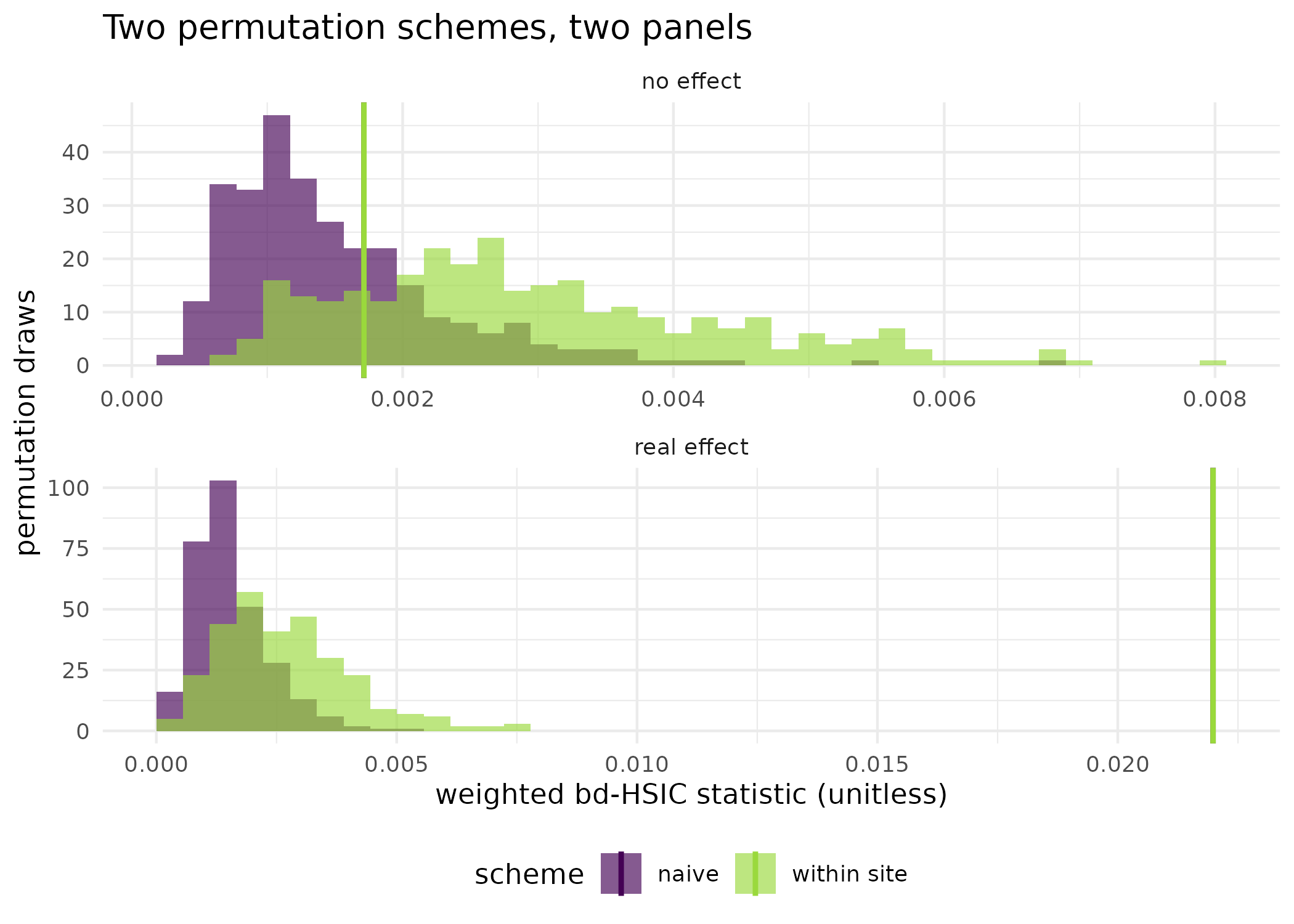

Permutation null distributions under the two schemes, on the panel with a real effect and on the panel without one, with the observed statistic marked in each. Shuffling within sites holds the site effects fixed, which changes the shape of the null the observed statistic is scored against; the naive scheme shuffles those effects into the null.

cluster_df <- data.frame(
  site = names(fit_site$per_cluster_statistic),
  statistic = as.numeric(fit_site$per_cluster_statistic),
  stringsAsFactors = FALSE
)
ggplot2::ggplot(
  cluster_df, ggplot2::aes(x = site, y = statistic)
) +
  ggplot2::geom_col(fill = "#3b528b") +
  ggplot2::geom_hline(
    yintercept = mean(cluster_df$statistic, na.rm = TRUE),
    colour = "#FDE725", linewidth = 0.9, linetype = "dashed"
  ) +
  ggplot2::labs(
    x = "site", y = "weighted bd-HSIC within site (unitless)",
    title = "Stratified contributions, site by site"
  ) +
  ggplot2::theme_minimal() +
  ggplot2::theme(axis.text.x = ggplot2::element_text(angle = 45,
                                                     hjust = 1))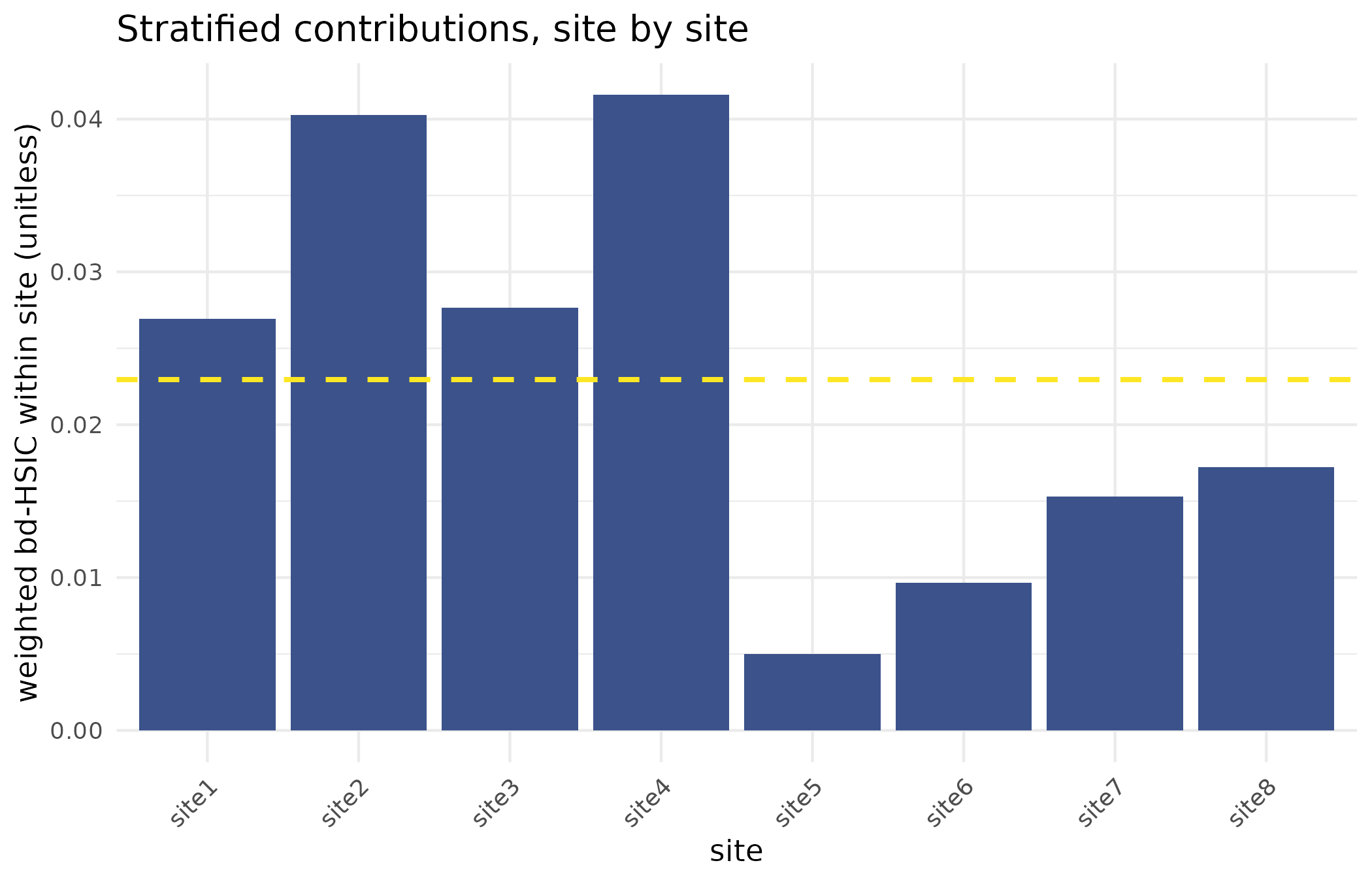

Weighted bd-HSIC computed inside each site on the panel with a real effect, with the mean across sites marked. A site whose stratified statistic dwarfs the rest is a candidate for follow-up, either as genuine site-specific effect modification or as a data-quality problem.

Read

On the panel with a real effect both schemes reject: the naive scheme gives a p-value of 0.0033 and the within-site scheme 0.0033, against the same observed statistic of 0.022, because the statistic does not depend on the permutation scheme. What differs is the null it is scored against, and the figure shows that directly: the naive null has a standard deviation of 0.00081 against 0.00136 for the within-site null, and a mean of 0.00154 against 0.00270: holding the site effects fixed shifts the whole null upward and widens it.

On the panel with the effect removed the two schemes give p-values of 0.32 (naive) and 0.8 (within site) against an observed statistic of 0.00171. Both decline to reject, which is the right answer on a panel built with no effect. One draw is not a type-I error rate: what this pair of runs shows is the mechanism, that the two schemes construct different nulls from identical data, and not a measured false-positive rate for either. Establishing that would need the whole panel regenerated many times over, which is a simulation study and not a vignette.

The stratified breakdown is the diagnostic worth keeping. Across the 8 sites with enough test observations to score, the within-site statistic runs from 0.005 to 0.0416, a factor of 8 between the quietest site and the loudest. The second figure shows the spread. A panel in which one site towers over the rest is telling you something the pooled verdict does not: either the effect is real only there, or that site’s data need looking at.

Limits

This is a synthetic panel with balanced sites and one level of nesting, and every result above is a single run. The within-site scheme needs at least two test observations per cluster, and the test split takes only part of the sample, so small clusters are reported as NA in per_cluster_statistic and contribute the identity permutation to the null; a design of paddocks with three to five plots each has little within-cluster permutation power and is usually better pooled to the site. The per-cluster statistics are reported on the raw scale and are not weighted by cluster size, so an unbalanced panel needs a size-weighted summary computed outside the function before the sites are compared. The choice of clustering level is an assumption about exchangeability, not a fact the data can supply: within-site permutation assumes plots inside a site are exchangeable, which a systematic within-site layout would break. Finally, everything the vignette Does the treatment cause the outcome, or do they share a cause? says about the density-ratio step applies unchanged here, including the effective-sample-size floor.

Choosing the scheme

Where the observations are genuinely independent and the design has no grouping, leave permutation at "auto" and supply no cluster_id: the propensity-similarity clustering is the intended default. Where the design has sites, seasons or paddocks that the covariates do not fully explain, supply cluster_id at the level you are willing to call exchangeable, and take the within-cluster scheme it activates. permutation = "naive" is for the case where within-cluster independence is plausible on other grounds and maximum power matters more, which is rare in a field trial.

Notes on practice

Cluster size. Within-cluster permutation needs at least two test observations per cluster, where the test split is one minus split_ratio of the sample. Clusters below that appear as NA in the stratified breakdown.

Many small clusters. Permutation power falls with cluster size. Pooling to a coarser level, site rather than paddock, is usually the better trade.

Imbalanced designs. Combine the per-cluster statistics with the cluster sizes yourself if a size-weighted summary is what the report needs.

What to read next

Does the treatment cause the outcome, or do they share a cause? introduces the backdoor-adjusted test and its density-ratio step, and is the place to start if bd-HSIC is new. When plots sit inside farms applies the same clustering idea to the doubly robust distributional tests, with a within-cluster and between-cluster decomposition this vignette does not compute. Choosing a density-ratio backend covers the adjustment step whose weights also determine the default clustering.

References

Hu, R., Sejdinovic, D., & Evans, R. J. (2024). A kernel test for causal association via noise contrastive backdoor adjustment. Journal of Machine Learning Research, 25(160), 1-56.

Reproduce

Seed 101 for the synthetic panel and for the null variant; seed = 1L passed to every test so the density-ratio fit and the permutation draws are fixed. Package versions follow.

sessionInfo()
#> R version 4.6.1 (2026-06-24)
#> Platform: x86_64-pc-linux-gnu
#> Running under: Ubuntu 24.04.5 LTS
#> 
#> Matrix products: default
#> BLAS:   /usr/lib/x86_64-linux-gnu/openblas-pthread/libblas.so.3 
#> LAPACK: /usr/lib/x86_64-linux-gnu/openblas-pthread/libopenblasp-r0.3.26.so;  LAPACK version 3.12.0
#> 
#> locale:
#>  [1] LC_CTYPE=C.UTF-8       LC_NUMERIC=C           LC_TIME=C.UTF-8       
#>  [4] LC_COLLATE=C.UTF-8     LC_MONETARY=C.UTF-8    LC_MESSAGES=C.UTF-8   
#>  [7] LC_PAPER=C.UTF-8       LC_NAME=C              LC_ADDRESS=C          
#> [10] LC_TELEPHONE=C         LC_MEASUREMENT=C.UTF-8 LC_IDENTIFICATION=C   
#> 
#> time zone: UTC
#> tzcode source: system (glibc)
#> 
#> attached base packages:
#> [1] stats     graphics  grDevices utils     datasets  methods   base     
#> 
#> other attached packages:
#> [1] kernR_0.10.0.9000
#> 
#> loaded via a namespace (and not attached):
#>  [1] vctrs_0.7.3         cli_3.6.6           knitr_1.52         
#>  [4] rlang_1.3.0         xfun_0.61           otel_0.2.0         
#>  [7] generics_0.1.4      S7_0.2.2            textshaping_1.0.5  
#> [10] data.table_1.18.6.1 jsonlite_2.0.0      labeling_0.4.3     
#> [13] glue_1.8.1          htmltools_0.5.9     PESTO_0.11.1.9000  
#> [16] ragg_1.5.2          sass_0.4.10         scales_1.4.0       
#> [19] rmarkdown_2.32      grid_4.6.1          evaluate_1.0.5     
#> [22] jquerylib_0.1.4     fastmap_1.2.0       yaml_2.3.12        
#> [25] lifecycle_1.0.5     compiler_4.6.1      RColorBrewer_1.1-3 
#> [28] fs_2.1.0            Rcpp_1.1.2          farver_2.1.2       
#> [31] systemfonts_1.3.2   digest_0.6.39       viridisLite_0.4.3  
#> [34] R6_2.6.1            bslib_0.12.0        withr_3.0.3        
#> [37] tools_4.6.1         gtable_0.3.6        pkgdown_2.2.1      
#> [40] ggplot2_4.0.3       cachem_1.1.0        desc_1.4.3