Wiring your own simulator into PESTO

library(PESTO)

Why

My simulator is APSIM, one run takes about a minute, and I want to calibrate it from R against a handful of seasons of measured yield. The question is: how do I wire a simulator like that into PESTO without paying a file round-trip on every realisation, and what do I have to get right for the posterior that comes back to be worth anything? This vignette answers both. The wiring is a typed forward-model contract that any R function can satisfy, demonstrated end to end on problems that run in seconds; the thing to get right is the observation standard deviation, and the middle of this vignette measures exactly how wrong an answer becomes when it is set the way most people first set it.

What

pesto_ies_callback() is the in-process driver. pesto_ies() shells out to the pestpp-ies binary, which writes and reads control, ensemble and observation files between every realisation; for an R forward model, whether that is an apsimx wrapper for APSIM, a bridge to another language, or a fast synthetic test problem, the file round-trip is pure overhead. The callback driver keeps the same C++ ensemble kernel (ensemble_solution(), after Chen and Oliver 2013) and drives the outer loop in R, calling the forward model in process. For APSIM this is the difference between re-reading an .apsimx file for every realisation and holding the model in memory across the whole ensemble.

pesto_forward_model() is the typed contract a forward model travels in. A bare function(theta) -> obs is the quickest way in and carries no metadata: the driver cannot know the output dimension in advance, cannot run realisations in parallel, and cannot express a failure budget. The contract object declares all three, and pesto_evaluate() runs it. apsim_callback() builds one for APSIM through the apsimx package: a working copy of a template per realisation, parameter edits by a param_map, a run, and an extraction step.

pesto_multifidelity_model() stacks an ordered set of fidelity levels, cheapest first, so early iterations can explore on a coarse model and late ones sharpen against the expensive one; mf_control_variate() is the variance-minimising affine correction that lifts cheap outputs toward expensive ones. ode_forward_model() and its two specialisations, crop_growth_forward_model() and seir_forward_model(), are ready-made contracts for the large class of simulators that are a small system of ordinary differential equations rather than an executable. pesto_ies_filter() assimilates time-ordered observation windows one after another rather than in one batch, which is what an in-season update needs.

Two diagnostics run throughout. ensemble_spread_ess() is recorded on every iteration, and pesto_abstention() is the typed decline a reliability gate returns in place of a result.

Do

A synthetic recovery example

The problem below is synthetic: a linear forward model at a known truth with Gaussian noise, which is the cheapest way to check that a driver recovers what it should before a real simulator is attached.

set.seed(20260516L)

npar <- 4L
nobs <- 8L
nreal <- 120L
sigma <- 0.05

G <- matrix(rnorm(nobs * npar), nobs, npar)
theta_true <- c(1.0, -0.5, 2.0, 0.25)
y <- as.numeric(G %*% theta_true) + rnorm(nobs, sd = sigma)
names(y) <- paste0("o", seq_len(nobs))

# Forward model: any function taking an (nreal x npar) matrix and returning
# an (nreal x nobs) matrix.
forward <- function(theta) theta %*% t(G)

prior <- matrix(rnorm(nreal * npar), nreal, npar,
                dimnames = list(NULL, paste0("p", seq_len(npar))))

Six iterations. lambda is left at its default: under the default ES-MDA scheme the Marquardt damping is the inflation factor (alpha = lambda + 1) and is set by the schedule, so it is chosen for you rather than fixed by hand (see ?pesto_ies_callback).

fit <- pesto_ies_callback(
  forward_model  = forward,
  prior_ensemble = prior,
  obs            = y,
  obs_sd         = sigma,
  noptmax        = 6L,
  seed           = 42L,
  verbose        = FALSE
)

prior_rmse <- sqrt(mean((colMeans(prior) - theta_true)^2))
post_mean <- colMeans(as.matrix(fit$par_ensemble[, -1L]))
post_rmse <- sqrt(mean((post_mean - theta_true)^2))
round(c(prior_rmse = prior_rmse, posterior_rmse = post_rmse), 4)
#>     prior_rmse posterior_rmse 
#>         1.1300         0.0231
vec_mean_phi <- vapply(fit$iterations, `[[`, numeric(1L), "mean_phi")
round(vec_mean_phi, 3)
#> [1] 17452.123    25.006    13.566     9.622     7.592     5.924

tab_phi_wide <- data.table::dcast(
  fit$phi, iteration ~ realisation, value.var = "phi"
)
plot_phi(tab_phi_wide, show_reals = TRUE,
         title = "Misfit by iteration, synthetic recovery problem")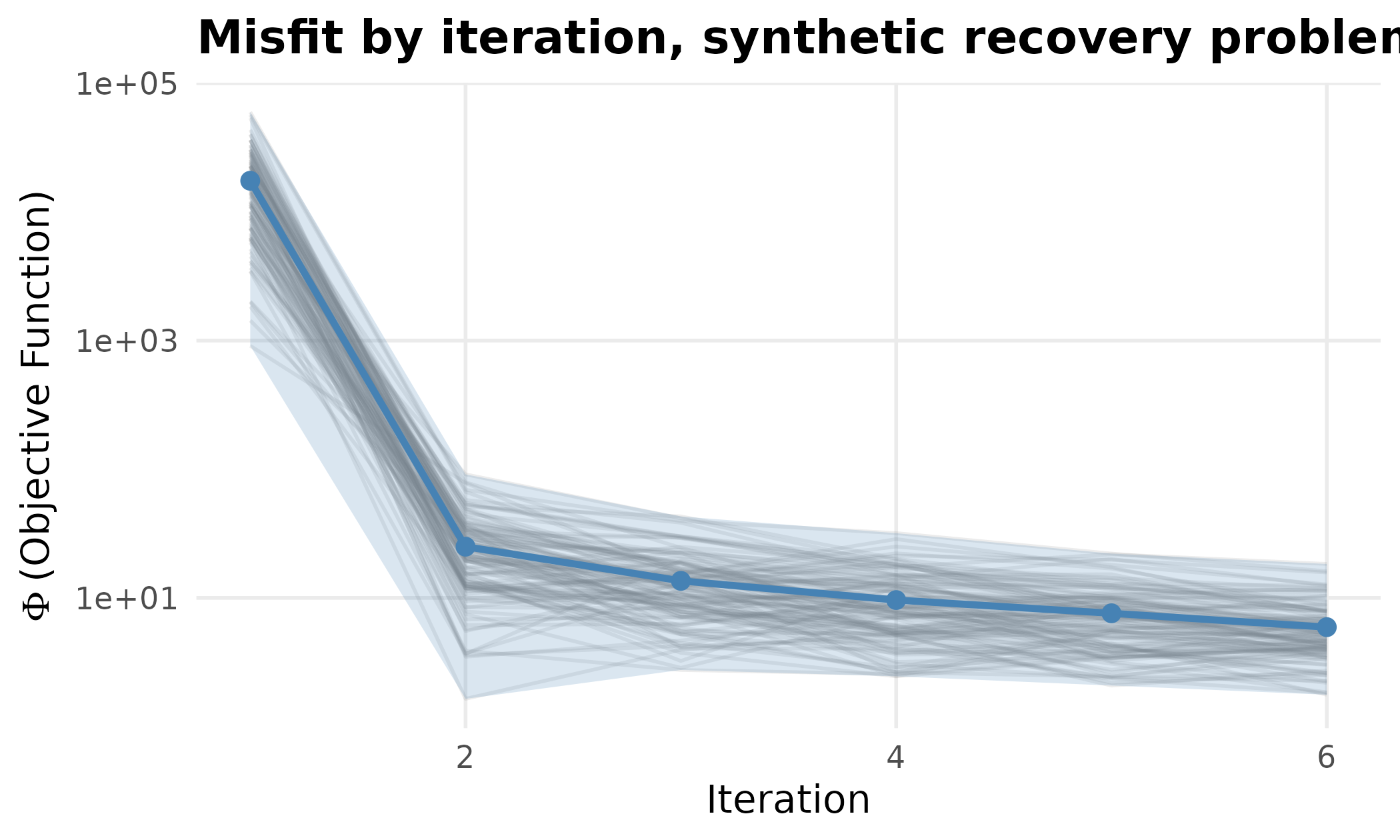

Objective function by iteration on the synthetic recovery problem. The ribbon spans the ensemble’s minimum to maximum misfit and each faint line is one realisation; the mean falls by nearly three orders of magnitude between the first and second iterations and then declines slowly.

The forward-model contract

pesto_forward_model() wraps the same callable in a typed contract that carries the metadata a bare function cannot. It is the single object both the native callback driver here and the classic .pst path are built to honour, so a forward model travels between modes unchanged.

fm <- pesto_forward_model(
  fn          = forward,
  n_obs       = nobs,
  param_names = paste0("p", seq_len(npar)),
  on_failure  = "na"
)

# A contract object is evaluated directly with pesto_evaluate(); the
# returned matrix carries the per-realisation failure count.
sim <- pesto_evaluate(fm, prior)
c(realisations = nrow(sim), outputs = ncol(sim),
  failures = attr(sim, "n_failures"))
#> realisations      outputs     failures 
#>          120            8            0

# Passing the contract to the driver is equivalent to passing the bare
# function: the bare form is auto-wrapped internally.
fit_typed <- pesto_ies_callback(fm, prior, y, sigma, noptmax = 6L,
                                seed = 42L, verbose = FALSE)
identical(
  as.matrix(fit_typed$par_ensemble[, -1L]),
  as.matrix(fit$par_ensemble[, -1L])
)
#> [1] TRUE

Parallel, fault-tolerant ensembles

For an expensive forward model, an APSIM ensemble especially, the realisations within one iteration are embarrassingly parallel. Build the contract with parallel = "multicore" and the evaluation engine dispatches rows across forked workers through parallel::mclapply(). For reproducible draws, set an "L'Ecuyer-CMRG" generator first, so each realisation receives an independent stream.

RNGkind("L'Ecuyer-CMRG")
set.seed(42L)

fm_par <- pesto_forward_model(
  fn       = forward,
  n_obs    = nobs,
  parallel = "multicore",
  n_cores  = 4L
)
fit_par <- pesto_ies_callback(fm_par, prior, y, sigma, noptmax = 6L)

The chunk above is shown rather than run, because forking inside a vignette build is not portable. A custom map_fn, any function shaped like lapply, is the escape hatch for a cross-platform or cluster backend. Failures are governed by on_failure, where "na" tolerates and "stop" aborts, and by max_fail_frac, which aborts once the fraction of failed realisations in a single evaluation exceeds the budget: a guardrail against an ensemble collapsing silently.

The number that decides whether to believe the answer

The single most consequential argument is obs_sd, the observation standard deviation, which sets the weights w = 1 / \sigma_{\mathrm{obs}}. It is also the easiest to get wrong in a way that fails silently. The failure mode is over-determination: conditioning the ensemble on a likelihood far tighter than the data deserve. The smoother then drives every realisation onto the same point, the posterior spread collapses, and the run reports an answer whose credible interval is far too narrow to be credible.

The usual route into the trap is statistical rather than a typo. Suppose each target observation is itself the mean of m field replicates. The replicate spread, the genuine measurement-plus-process noise a single modelled value must match, is \sigma. The standard error of that mean is \sigma / \sqrt{m}, smaller by a factor of \sqrt{m} and shrinking further as more plots are averaged. Passing the standard error as obs_sd tells the smoother the data pin the model roughly \sqrt{m} times more sharply than they do. The forward model cannot be that right, so the ensemble has nowhere to go but onto a single collapsed point.

m <- 40L
obs_se <- sigma / sqrt(m)   # the standard error of a 40-replicate mean

fit_ok <- pesto_ies_callback(
  forward, prior, y,
  obs_sd  = sigma,          # field-realistic replicate spread
  noptmax = 6L, seed = 42L, verbose = FALSE
)

fit_collapsed <- pesto_ies_callback(
  forward, prior, y,
  obs_sd  = obs_se,         # the over-precise likelihood, the trap
  noptmax = 6L, seed = 42L, verbose = FALSE
)

The collapse does not announce itself in the posterior mean. On this linear-Gaussian problem both runs recover the truth to three figures. It announces itself in the posterior spread, and in whether the credible interval still covers the truth.

spread <- function(fit) {
  mean(apply(as.matrix(fit$par_ensemble[, -1L]), 2L, sd))
}

coverage_90 <- function(fit, truth) {
  pe <- as.matrix(fit$par_ensemble[, -1L])
  lo <- apply(pe, 2L, quantile, 0.05)
  hi <- apply(pe, 2L, quantile, 0.95)
  mean(truth >= lo & truth <= hi)   # fraction of params inside the band
}

tab_two <- data.frame(
  Case = c("field-realistic", "over-precise (SE of a 40-replicate mean)"),
  `obs_sd` = c(sigma, obs_se),
  `Mean posterior SD` = c(spread(fit_ok), spread(fit_collapsed)),
  `Coverage of the 90% band (%)` = 100 * c(
    coverage_90(fit_ok, theta_true), coverage_90(fit_collapsed, theta_true)
  ),
  check.names = FALSE
)

The same problem and the same data under a field-realistic and an over-precise observation standard deviation.
Case	obs_sd	Mean posterior SD	Coverage of the 90% band (%)
field-realistic	0.0500	0.0341	100
over-precise (SE of a 40-replicate mean)	0.0079	0.0054	50

Where the boundary is

Two cases show that the failure exists. A sweep shows where it starts. The block below repeats the run at replicate counts from 1 to 160, each time passing the standard error of an m-replicate mean as obs_sd, and records two things: the mean posterior standard deviation, and how far the posterior mean sits from the truth measured in its own posterior standard deviations. A calibrated posterior puts the truth within about one of its own standard deviations; a collapsed one puts it many.

vec_m <- c(1L, 2L, 5L, 10L, 20L, 40L, 80L, 160L)
tab_boundary <- data.table::rbindlist(lapply(vec_m, function(mm) {
  fit_m <- pesto_ies_callback(
    forward, prior, y, obs_sd = sigma / sqrt(mm),
    noptmax = 6L, seed = 42L, verbose = FALSE
  )
  pe <- as.matrix(fit_m$par_ensemble[, -1L])
  par_sd <- apply(pe, 2L, sd)
  data.table::data.table(
    m = mm,
    obs_sd = sigma / sqrt(mm),
    post_sd = mean(par_sd),
    z = mean(abs(colMeans(pe) - theta_true) / par_sd),
    coverage = coverage_90(fit_m, theta_true)
  )
})) # ends the sweep over replicate counts

ggplot2::ggplot(
  tab_boundary, ggplot2::aes(x = m, y = z, colour = coverage)
) +
  ggplot2::geom_hline(yintercept = 1, linetype = "dashed",
                      colour = "grey40") +
  ggplot2::geom_line(colour = "grey60", linewidth = 0.8) +
  ggplot2::geom_point(size = 3.4) +
  ggplot2::scale_x_log10() +
  ggplot2::scale_y_log10() +
  ggplot2::scale_colour_viridis_c(
    name = "90% coverage", limits = c(0, 1), end = 0.9
  ) +
  ggplot2::labs(
    x = "replicates averaged into each observation (log scale)",
    y = "distance from truth, in posterior SDs (log scale)",
    title = "How over-precise an obs_sd can be before the answer misleads"
  ) +
  ggplot2::theme_minimal(base_size = 12)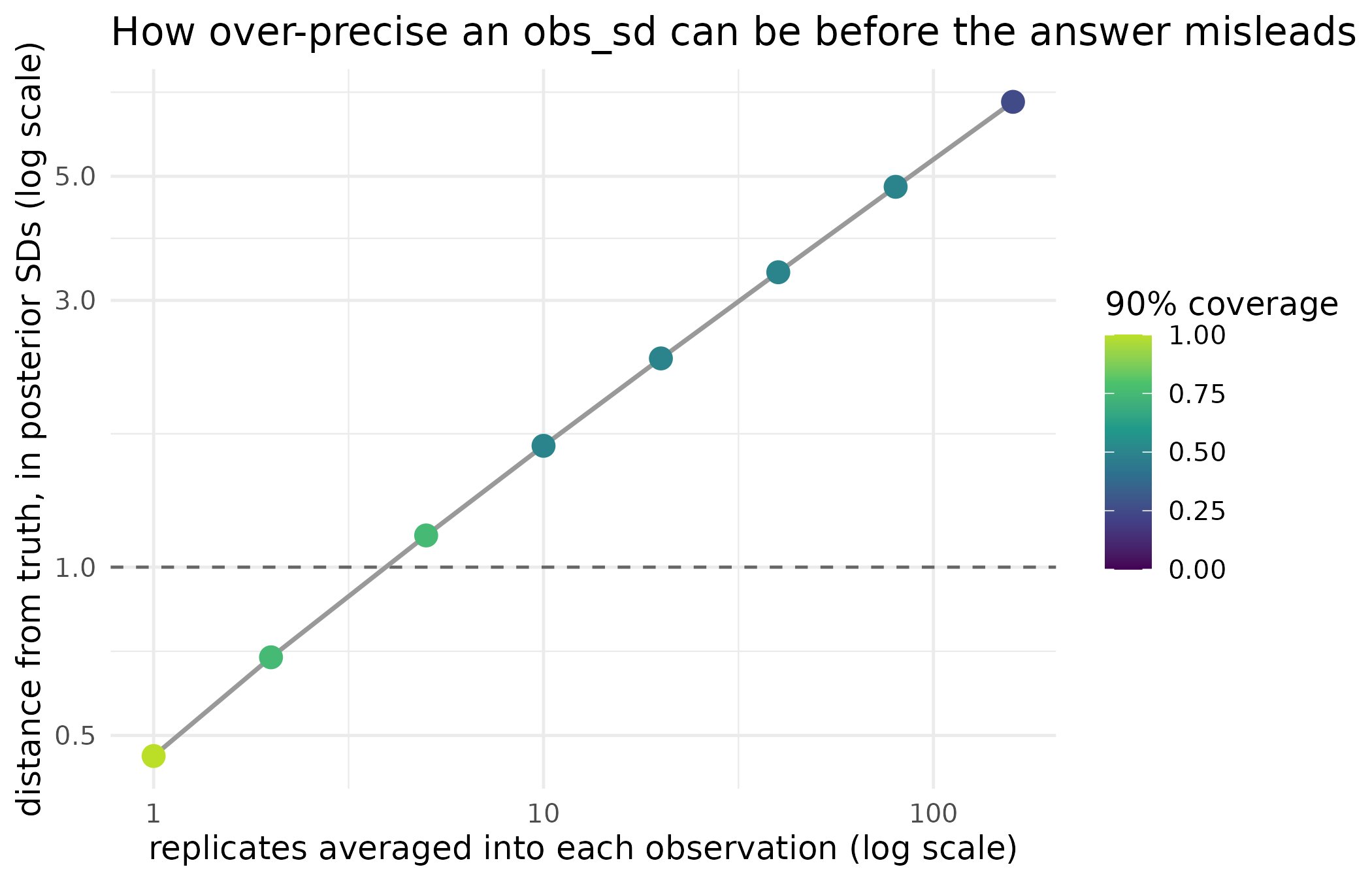

$The over-determination boundary. The horizontal axis is the number of replicates whose standard error was passed as obs_sd; the vertical axis is how far the posterior mean sits from the known truth, measured in posterior standard deviations. Point colour is the fraction of parameters whose 90 per cent credible band still covers the truth. The dashed line at one standard deviation is where a posterior stops being able to describe its own error, and everything to the right of the crossing is a run that reports false confidence.$

The over-determination boundary. The horizontal axis is the number of replicates whose standard error was passed as obs_sd; the vertical axis is how far the posterior mean sits from the known truth, measured in posterior standard deviations. Point colour is the fraction of parameters whose 90 per cent credible band still covers the truth. The dashed line at one standard deviation is where a posterior stops being able to describe its own error, and everything to the right of the crossing is a run that reports false confidence.

The same inversion at eight settings of obs_sd, each the standard error of a mean over m replicates of a spread of 0.05.
Replicates m	obs_sd passed	Mean posterior SD	Distance from truth (posterior SDs)	90% coverage (fraction)
1	0.0500	0.0341	0.4594	1.00
2	0.0354	0.0241	0.6899	0.75
5	0.0224	0.0152	1.1395	0.75
10	0.0158	0.0108	1.6481	0.50
20	0.0112	0.0076	2.3622	0.50
40	0.0079	0.0054	3.3683	0.50
80	0.0056	0.0038	4.7885	0.50
160	0.0040	0.0027	6.7951	0.25

PESTO does not gate this automatically: pesto_abstention()’s reason codes are not a closed set, and a caller who can measure the boundary can mint the gate. The function below is that gate, written against the sweep’s own statistic, and it returns a typed decline that a downstream tool recognises by class rather than by parsing a message.

gate_over_determination <- function(fit, truth, z_max = 1.5) {
  pe <- as.matrix(fit$par_ensemble[, -1L])
  par_sd <- apply(pe, 2L, sd)
  z <- mean(abs(colMeans(pe) - truth) / par_sd)
  if (z > z_max) {
    return(pesto_abstention(
      "over_determined",
      detail = sprintf(
        paste0("posterior mean sits %.1f posterior SDs from the reference, ",
               "above the tolerance of %.1f; obs_sd is too small"),
        z, z_max
      ),
      diagnostics = list(z = round(z, 2), mean_post_sd = mean(par_sd))
    ))
  }
  fit
}

is_pesto_abstention(gate_over_determination(fit_ok, theta_true))
#> [1] FALSE
gate_over_determination(fit_collapsed, theta_true)
#> $reason
#> [1] "over_determined"
#> 
#> $detail
#> [1] "posterior mean sits 3.4 posterior SDs from the reference, above the tolerance of 1.5; obs_sd is too small"
#> 
#> $diagnostics
#> $diagnostics$z
#> [1] 3.37
#> 
#> $diagnostics$mean_post_sd
#> [1] 0.005380416
#> 
#> 
#> $scope
#> [1] "call"
#> 
#> $abstained
#> [1] TRUE
#> 
#> attr(,"class")
#> [1] "pesto_abstention"

What the spread-ESS diagnostic can and cannot see

ensemble_spread_ess() is logged on every iteration as spread_ess and as the ratio spread_ess_ratio, and it is worth being precise about its reach. It is the spectral participation ratio of the parameter anomaly covariance, the effective number of variance-carrying directions, so it detects the shape of a collapse: variance draining into a few directions. It is a ratio of eigenvalue sums, hence invariant to a global rescaling of the anomalies, so a spread that is uniformly too small in every direction is invisible to it. The two runs above differ in exactly that way.

ess_ratio <- function(fit) {
  vapply(fit$iterations, `[[`, numeric(1L), "spread_ess_ratio")
}
tab_ess <- rbind(
  `field-realistic` = round(ess_ratio(fit_ok), 3),
  `over-precise`    = round(ess_ratio(fit_collapsed), 3)
)
tab_ess
#>                  [,1]  [,2]  [,3]  [,4]  [,5]  [,6]
#> field-realistic 0.556 0.518 0.503 0.508 0.504 0.483
#> over-precise    0.550 0.522 0.504 0.509 0.507 0.487

Read spread_ess_ratio as the directional-collapse diagnostic it is, and read the coverage column of the boundary table as the calibration check. They answer different questions and only the second catches a mis-specified obs_sd.

The fix is to set obs_sd to the uncertainty the modelled value must actually reproduce, the replicate-level measurement-plus-process spread, never the standard error of an average:

Use the replicate standard deviation \sigma, not \sigma / \sqrt{m}, when the target is a mean over m measurements.
Fold structural model discrepancy into obs_sd. The forward model is an approximation, and the likelihood should not pretend it matches reality more tightly than the model can.
When in genuine doubt, err wide. An over-wide obs_sd leaves spread on the table and under-uses the data; an over-narrow one destroys the ensemble and reports false confidence.

When over-determination is unavoidable, with many observations and few realisations, the covariance inflation and localisation countermeasures in My posterior looks too confident: is the ensemble collapsing? replenish the collapsing spread rather than only diagnosing it. A correctly specified obs_sd is the first line of defence and those countermeasures the second.

Driving APSIM through `apsim_callback()`

The adapter wraps apsimx so each realisation gets its own working copy of an APSIM template, parameter edits per param_map, a run, and an extraction step. What it returns matches what pesto_ies_callback() expects.

The apsimx package is installed here but no APSIM executable is advertised through PESTO_APSIM_EXE, so the block below is shown rather than run.

library(apsimx)   # >= 2.7.0 from CRAN; needs a working APSIM Next Gen

forward_apsim <- apsim_callback(
  template  = "wheat_wagga.apsimx",
  param_map = list(
    RUE = "Wheat.Leaf.Photosynthesis.RUE.FixedValue",
    CN2 = "Soil.SoilWater.CN2Bare"
  ),
  output_extractor = function(sim) {
    # sim is the data.frame of report-table variables.
    as.numeric(sim$Wheat.Grain.Total.Wt)
  }
)

prior_apsim <- cbind(
  RUE = runif(40L, 1.0, 2.0),
  CN2 = runif(40L, 60, 90)
)

fit_apsim <- pesto_ies_callback(
  forward_model  = forward_apsim,
  prior_ensemble = prior_apsim,
  obs            = c(y_2018 = 4500, y_2019 = 5200, y_2020 = 4900),
  obs_sd         = 250,
  noptmax        = 4L
)

Per-realisation APSIM crashes, whether a corrupt configuration, a solver divergence or a missing report variable, are caught by the adapter and emerge as NA rows. The driver’s default on_failure = "na" carries those realisations forward unchanged so the ensemble survives partial failure; on_failure = "stop" aborts as soon as one row is missing.

The closure writes each realisation to its own uniquely named working file, so it is safe to evaluate in parallel: wrap it in a pesto_forward_model(parallel = "multicore") exactly as above and the ensemble runs across forked workers, each invoking APSIM on its own input. Start with a modest n_cores, because the thread safety of apsimx itself under heavy ensemble load has not been independently characterised. For pure-R synthetic models the serial loop is already fast enough that the overhead is dominated by ensemble_solution().

Multi-fidelity calibration

Process-based crop models expose a cost-accuracy dial: a daily time step with a lite soil profile is cheap, a sub-daily step with the full profile is expensive. pesto_multifidelity_model() makes that dial first class. It bundles an ordered stack of fidelity levels, cheapest first, and the driver picks a level per iteration through a fidelity_schedule, so early iterations explore cheaply and late ones sharpen against the expensive truth. The final ensemble is always refreshed at the highest fidelity.

# Cheap level: the linear model with a small systematic bias.
# Expensive level: the unbiased truth.
cheap_fn <- function(theta) theta %*% t(G) + 0.30
expensive_fn <- forward

mf <- pesto_multifidelity_model(
  levels = list(
    pesto_forward_model(fn = cheap_fn,     n_obs = nobs, fidelity = 0L),
    pesto_forward_model(fn = expensive_fn, n_obs = nobs, fidelity = 1L)
  ),
  costs = c(1, 25)   # the expensive level is about 25 times dearer per run
)

# Ramp: two cheap iterations, then four expensive ones.
fit_mf <- pesto_ies_callback(
  forward_model     = mf,
  prior_ensemble    = prior,
  obs               = y,
  obs_sd            = sigma,
  noptmax           = 6L,
  fidelity_schedule = c(0L, 0L, 1L, 1L, 1L, 1L),
  seed              = 42L,
  verbose           = FALSE
)

mf_rmse <- sqrt(mean(
  (colMeans(as.matrix(fit_mf$par_ensemble[, -1L])) - theta_true)^2
))
round(c(single_fidelity_rmse = post_rmse, multi_fidelity_rmse = mf_rmse), 4)
#> single_fidelity_rmse  multi_fidelity_rmse 
#>               0.0231               0.0968

When the cheap level is run over the whole ensemble and the expensive level over only a subset, mf_control_variate() lifts the cheap outputs toward the expensive ones with the variance-minimising affine correction, which is the plug-in primitive for a surrogate cascade:

sub <- seq_len(20L)
low_all <- pesto_evaluate(mf, prior, level = 0L)
low_sub <- low_all[sub, , drop = FALSE]
high_sub <- pesto_evaluate(mf, prior[sub, , drop = FALSE], level = 1L)

corrected <- mf_control_variate(low_all, high_sub, low_sub)
high_all <- pesto_evaluate(mf, prior, level = 1L)
gap_before <- mean(abs(low_all - high_all))
gap_after <- mean(abs(corrected - high_all))
signif(c(mean_gap_before = gap_before, mean_gap_after = gap_after), 3)
#> mean_gap_before  mean_gap_after 
#>        3.00e-01        3.39e-17

Simulators that are systems of equations

Not every simulator sits behind an executable. A very large class, crop growth, epidemic dynamics, nutrient or solute transport and pharmacokinetics among them, is a small system of ordinary differential equations integrated forward in time with the observation vector read off the state trajectory. PESTO ships these as templates returning the same typed contract as everything above, so they plug straight into the driver, the multi-fidelity stack and the manifest emitter. Integration is a self-contained fixed-step fourth-order Runge-Kutta scheme by default, with a solver = "desolve" path delegating to the deSolve package for stiff systems.

The generic builder is ode_forward_model(): supply the derivative function, the initial state, the time grid, and which parameter columns the model consumes. crop_growth_forward_model() is the logistic dry-matter curve \mathrm{d}B / \mathrm{d}t = r B (1 - B / b_{\max}), the canonical sigmoid description of seasonal biomass, calibrating r, b_{\max} and the starting biomass against an observed biomass series.

times <- seq(0, 120, by = 15)
crop <- crop_growth_forward_model(times = times)

# Simulate a biomass series at a known parameter, then add field noise.
theta_crop <- c(r = 0.06, b_max = 1400, b0 = 20)
biomass <- as.numeric(pesto_evaluate(
  crop, matrix(theta_crop, nrow = 1L,
               dimnames = list(NULL, names(theta_crop)))
))
y_crop <- biomass + rnorm(length(biomass), sd = 20)
names(y_crop) <- paste0("t", seq_along(y_crop))

prior_crop <- cbind(
  r     = runif(120L, 0.02, 0.12),
  b_max = runif(120L, 900, 2000),
  b0    = runif(120L, 5, 60)
)
fit_crop <- pesto_ies_callback(crop, prior_crop, y_crop, obs_sd = 20,
                              noptmax = 8L, seed = 42L, verbose = FALSE)
post_crop <- colMeans(
  as.matrix(fit_crop$par_ensemble[, -1L])
)[names(theta_crop)]

Recovery of the logistic growth parameters from a noisy biomass series.
Parameter	Unit	Truth	Posterior mean
r	per day	0.06	0.062
b_max	g/m2	1400.00	1374.369
b0	g/m2	20.00	19.906

seir_forward_model() is the closed-population susceptible-exposed-infectious-recovered epidemic model, calibrating the transmission, latency and recovery rates against an observed infectious prevalence curve. The reproduction number R_0 = \beta / \gamma is the summary an outbreak curve identifies most sharply.

days <- seq(0, 60, by = 5)
seir <- seir_forward_model(times = days, n_pop = 1000, i0 = 1)

theta_seir <- c(beta = 0.6, sigma = 0.2, gamma = 0.1)
prevalence <- as.numeric(pesto_evaluate(
  seir, matrix(theta_seir, nrow = 1L,
               dimnames = list(NULL, names(theta_seir)))
))
y_seir <- prevalence + rnorm(length(prevalence), sd = 3)
names(y_seir) <- paste0("d", seq_along(y_seir))

prior_seir <- cbind(
  beta  = runif(200L, 0.3, 0.9),
  sigma = runif(200L, 0.1, 0.4),
  gamma = runif(200L, 0.05, 0.2)
)
fit_seir <- pesto_ies_callback(seir, prior_seir, y_seir, obs_sd = 3,
                               noptmax = 10L, seed = 42L, verbose = FALSE)
post_seir <- colMeans(
  as.matrix(fit_seir$par_ensemble[, -1L])
)[names(theta_seir)]
r0_truth <- theta_seir[["beta"]] / theta_seir[["gamma"]]
r0_post <- post_seir[["beta"]] / post_seir[["gamma"]]
round(c(R0_truth = r0_truth, R0_posterior = r0_post), 2)
#>     R0_truth R0_posterior 
#>         6.00         6.02

Because both templates return a pesto_forward_model(), the coarse and fine fidelity trick from the previous section applies verbatim: build one template at a coarse n_steps and one at a fine n_steps, stack them in a pesto_multifidelity_model(), and ramp the integration resolution across iterations.

Assimilating a season as it happens

pesto_ies_callback() is a smoother: it assimilates every observation in one batch. For an in-season setting, where a season’s observations arrive over time and the parameter posterior is wanted as the season progresses rather than only at harvest, pesto_ies_filter() is the filter. It assimilates time-ordered observation windows one after another against the same static calibration parameters, and each window’s posterior becomes the next window’s prior, so information accrues and the posterior tightens window by window.

# Split the eight observations into three temporal windows, standing in for
# early, mid and late season.
windows <- list(1:3, 4:6, 7:8)

fit_seq <- pesto_ies_filter(
  forward_model  = forward,
  prior_ensemble = prior,
  obs            = y,
  obs_sd         = sigma,
  windows        = windows,
  seed           = 42L,
  verbose        = FALSE
)

sd_trace <- vapply(fit_seq$windows, function(w) mean(w$par_sd), numeric(1L))
tab_filter <- data.frame(
  Window = seq_along(sd_trace),
  `Observations assimilated` = vapply(
    fit_seq$windows, function(w) length(w$obs_indices), integer(1L)
  ),
  `Mean parameter SD` = sd_trace,
  check.names = FALSE
)

The filter’s posterior spread after each window. The value of the filter is the trajectory, not only the endpoint.
Window	Observations assimilated	Mean parameter SD
1	3	0.4119
2	3	0.0399
3	2	0.0340

A multi-fidelity stack plugs in through fidelity_schedule, one level per window, so a run can be cheap early and sharpen late, and the result wraps into the same manifest contract through as_manifest(), tagged method = "ies_filter".

When to prefer the `.pst` path instead

Use pesto_ies() and the classic control-file path when the forward model lives behind a non-R executable that PEST++ can drive directly through its template and instruction files; when bit-for-bit compatibility with pestpp-ies behaviour is needed, for instance to cross-validate against an existing PEST++ workflow; or when a pestpp-ies feature not yet exposed by the R driver is required, such as the full lambda line search, regularisation modes or Tikhonov priors. Otherwise the callback driver is faster to iterate, easier to debug, and avoids per-realisation file exchange entirely.

Read

The driver recovers what it should. Posterior root-mean-square error to the truth is 0.0231 against a prior figure of 1.13, a reduction of a factor of 49, and the ensemble mean misfit falls from 17,450 to 5.92 across 6 iterations. Handing the driver a typed contract instead of a bare function returns a posterior ensemble identical to the bare-function run, which is the property that lets a forward model move between calling conventions unchanged.

The obs_sd sweep is the centre of this vignette. Passing the replicate spread gives a mean posterior standard deviation of 0.0341 and a 90 per cent band that covers 100 per cent of the parameters. Passing the standard error of a 40-replicate mean, about 6 times smaller, shrinks the posterior standard deviation to 0.00538, roughly 16 per cent of the well-specified run, and drops coverage to 50 per cent. The figure shows that this is not a cliff but a slope with a crossing point: the distance from the truth in posterior standard deviations rises from 0.46 at one replicate to 6.8 at 160, crossing one standard deviation between 2 and 5 replicates. Beyond that crossing the posterior can no longer describe its own error, and coverage falls from 100 per cent to 25 per cent across the sweep.

The spread-ESS trace explains why a diagnostic is not automatically a safeguard. The two runs’ trajectories sit within 0.005 of each other at every iteration even though one ensemble’s spread is a small fraction of the other’s, because the statistic is invariant to a global rescaling of the anomalies. That is the case for reading it as a directional-collapse diagnostic and reading coverage as the calibration check. Because PESTO does not gate on the sweep’s statistic itself, the gate_over_determination() function above mints the decline a caller wants: applied to the well-specified run it returns the run, and applied to the collapsed one it returns a pesto_abstention with reason over_determined, which a downstream tool recognises by class rather than by reading a message.

The remaining machinery does what it claims, with one price worth naming. The multi-fidelity stack, running two cheap iterations before four expensive ones, reaches a posterior root-mean-square error of 0.0968 against the single-fidelity run’s 0.0231: still far better than the prior, but a factor of 4.2 worse than spending every iteration on the expensive level. Two of six iterations spent on a biased model is not free, and whether that trade is worth taking depends on the cost ratio between the levels, which here was declared as 25 to 1. The control-variate correction, by contrast, is close to exact on this problem: the mean absolute gap between the cheap and expensive levels falls from 0.3 to 3e-17, which is machine precision, because the cheap level’s bias is a constant offset and an affine correction removes a constant offset exactly. The logistic growth template recovers a ceiling of 1374 g/m2 against a truth of 1400 and a growth rate of 0.062 against 0.06. The epidemic template recovers a reproduction number of 6.02 against a truth of 6. The filter tightens the posterior window by window, from a mean parameter standard deviation of 0.412 after the first window to 0.034 after the third, which is the trajectory an in-season user wants rather than the endpoint alone.

Limits

Every problem run here is synthetic, and the central one is linear and Gaussian, so the recovery it demonstrates is the easiest case there is; nothing in this vignette establishes that a real APSIM calibration converges or that its posterior is calibrated, which is what Can PESTO recover APSIM’s own parameters? takes up on a simulator-backed run and on real measured biomass. The APSIM adapter is shown and not executed, so its code path is documented rather than exercised here, and the parallel evaluation path is likewise shown rather than run. The over-determination boundary is measured against a known truth, which a real calibration does not have: on a real problem the same diagnosis has to be made from held-out predictive coverage rather than from distance to a truth, and the minted gate above would have to be rewritten around that substitute. The boundary’s crossing point is a property of this problem’s parameter count, ensemble size and design matrix, not a universal threshold, so the number to carry away is the method rather than the value. Multi-fidelity is demonstrated with a cheap level that differs from the expensive one by a constant offset, which is the friendliest possible discrepancy; a cheap level whose bias varies with the parameters would behave differently and is not tested here. The filter is run on observations split into windows after the fact rather than arriving over a real season, so it shows the mechanism and not the operational case.

What to read next

Can PESTO recover APSIM’s own parameters? is this vignette’s counterpart on a real simulator: a synthetic-truth recovery experiment against the bundled APSIM Wheat example, then a calibration to real measured biomass cross-checked against an independent optimiser. My posterior looks too confident: is the ensemble collapsing? is the second line of defence against a narrow posterior, and separates finite-ensemble collapse from the mis-specification diagnosed here. When can a surrogate stand in for the simulator? is the other way to spend fewer expensive model calls. Handing an ensemble to somebody else documents the record a finished run emits. Is PESTO the same algorithm as the tools it descends from? measures what the in-process driver buys against the file-coupled binaries.

References

Chen, Y., & Oliver, D. S. (2013). Levenberg-Marquardt forms of the iterative ensemble smoother for efficient history matching and uncertainty quantification. Computational Geosciences, 17(4), 689-703.
Emerick, A. A., & Reynolds, A. C. (2013). Ensemble smoother with multiple data assimilation. Computers & Geosciences, 55, 3-15.
Glasserman, P. (2003). Monte Carlo Methods in Financial Engineering. Springer, New York.
Holzworth, D., et al. (2014). APSIM: evolution towards a new generation of agricultural systems simulation. Environmental Modelling & Software, 62, 327-350.
Kennedy, M. C., & O’Hagan, A. (2000). Predicting the output from a complex computer code when fast approximations are available. Biometrika, 87(1), 1-13.

Reproduce

Seed 20260516 sets the design matrix, the truth and the observation noise; seed 42 is passed to every pesto_ies_callback() and pesto_ies_filter() call, where it fixes the per-realisation observation perturbation, so all runs are compared on identical perturbed data. No external simulator or binary is used. Package versions follow.

sessionInfo()
#> R version 4.6.1 (2026-06-24)
#> Platform: x86_64-pc-linux-gnu
#> Running under: Ubuntu 24.04.5 LTS
#> 
#> Matrix products: default
#> BLAS:   /usr/lib/x86_64-linux-gnu/openblas-pthread/libblas.so.3 
#> LAPACK: /usr/lib/x86_64-linux-gnu/openblas-pthread/libopenblasp-r0.3.26.so;  LAPACK version 3.12.0
#> 
#> locale:
#>  [1] LC_CTYPE=C.UTF-8       LC_NUMERIC=C           LC_TIME=C.UTF-8       
#>  [4] LC_COLLATE=C.UTF-8     LC_MONETARY=C.UTF-8    LC_MESSAGES=C.UTF-8   
#>  [7] LC_PAPER=C.UTF-8       LC_NAME=C              LC_ADDRESS=C          
#> [10] LC_TELEPHONE=C         LC_MEASUREMENT=C.UTF-8 LC_IDENTIFICATION=C   
#> 
#> time zone: UTC
#> tzcode source: system (glibc)
#> 
#> attached base packages:
#> [1] stats     graphics  grDevices utils     datasets  methods   base     
#> 
#> other attached packages:
#> [1] PESTO_0.11.1.9000
#> 
#> loaded via a namespace (and not attached):
#>  [1] bit_4.6.0           gtable_0.3.6        jsonlite_2.0.0     
#>  [4] compiler_4.6.1      Rcpp_1.1.2          xml2_1.6.0         
#>  [7] blob_1.3.0          jquerylib_0.1.4     systemfonts_1.3.2  
#> [10] scales_1.4.0        textshaping_1.0.5   apsimx_2.8.271     
#> [13] yaml_2.3.12         fastmap_1.2.0       ggplot2_4.0.3      
#> [16] R6_2.6.1            labeling_0.4.3      knitr_1.52         
#> [19] desc_1.4.3          DBI_1.3.0           bslib_0.12.0       
#> [22] RColorBrewer_1.1-3  rlang_1.3.0         cachem_1.1.0       
#> [25] xfun_0.61           fs_2.1.0            sass_0.4.10        
#> [28] S7_0.2.2            bit64_4.8.6         otel_0.2.0         
#> [31] memoise_2.0.1       viridisLite_0.4.3   RSQLite_3.53.3     
#> [34] cli_3.6.6           pkgdown_2.2.1       withr_3.0.3        
#> [37] digest_0.6.39       grid_4.6.1          lifecycle_1.0.5    
#> [40] vctrs_0.7.3         evaluate_1.0.5      glue_1.8.1         
#> [43] data.table_1.18.6.1 farver_2.1.2        ragg_1.5.2         
#> [46] rmarkdown_2.32      tools_4.6.1         htmltools_0.5.9

Why